Economics
2iec & 1iec
Overview of 2iec
- Basic economic ideas and resource allocation
- The price system and the microeconomy
- Government microeconomic intervention
- The macroeconomy
- Government macroeconomic intervention
- International economic issues
Overview of 1iec
- The price system and the microeconomy
- Government microeconomic intervention
- The macroeconomy
- Government macroeconomic intervention
- International economic issues
Structured Writing - Simple Model

Structured Writing - Intermediate Model

Structured Writing - Advanced Model

sample essays on ...
- monopoly
- labour supply
- protectionism
- globalisation
- interest rate
- development
monopoly
- Read: Tesla holds 80% of US EV market despite losing federal tax credit
- Evaluate whether a monopoly is likely to operate efficiently. Refer to at least one monopoly of your choice.
labour supply
- Read: The five UK sectors grappling with acute labour shortages
- Evaluate the factors that might influence the supply of labour in an occupation of your choice.
protectionism
- Read: IMF warns there is 'limited ammunition' to fight recession
- Evaluate the likely impact of an increase in protectionism on the global economy.
globalisation
- Read: The modern era of globalisation is in danger
- Evaluate the likely impact of globalisation on the global economy.
interest rates
- Evaluate the microeconomic and macroeconomic effects of decreasing interest rates in Kenya, or another developing country of your choice.
development
- Evaluate the microeconomic and macroeconomic strategies that could be used to promote development in Kenya, or another developing country of your choice.
Flipped classroom - Video ressources
List of videos on economic conceptsStudy plan (2iec)
Part 1: Basic economic ideas and resource allocation
- Scarcity, choice and opportunity cost
- Economic methodology
- Factors of production
- Resource allocation in different economic systems
- Production possibility curves
- Classification of goods and services
Chapter 1: Scarcity, choice and opportunity cost
- fundamental economic problem
- resources
- wants
- needs
- scarcity
- choice
- factors of production
- firm
- opportunity cost
Chapter 1: Scarcity, choice and opportunity cost
- wants
- needs
- resources
- economic problem
- opportunity cost
- scarcity and choice
fundamental economic problem
- scarce resources ...
- ... but unlimited wants.
resources
- inputs available ...
- ... for the production ...
- ... of goods and services
wants
- the goods and services ...
- ... that people may like to have ...
- ... but are not always realised
needs
- things that are necessary for survival ...
- ... such as food
scarcity
- a situation ...
- ... in which wants and needs ...
- ... are greater than ...
- ... the resources available
choice
- resources are scarce ...
- ... so individuals, firms and governments ...
- ... have to consider alternatives
factors of production
- resources or inputs ...
- ... available in an economy ...
- ... that are used in the production ...
- ... of goods and services
firm
- any business ...
- ... that hires factors of production ...
- ... to produce good and services
opportunity cost
- the cost expressed ...
- ... in terms of ...
- ... the next best alternative forgone ...
- ... when a choice is made
basic economic problem
Credit: "Pittsburgh Homeless" by "daveyinn"/Flickr Creative Commons, CC BY 2.0
choices and tradeoffs
Credit: modification of "College of DuPage Commencement 2018 107" by COD Newsroom/Flickr, CC BY 2.0
budget constraint
Each point on the budget constraint represents a combination of burgers and bus tickets whose total cost adds up to Alphonso's budget of $10. The relative price of burgers and bus tickets determines the slope of the budget constraint. All along the budget set, giving up one burger means gaining four bus tickets.
resources
- inputs available ...
- ... for the production of goods and services
opportunity cost
scarcity
- situation that arises because
- people have unlimited wants
- in the face of limited resources
scarcity and choice
- choices are made
- by different agents : households, firms, government, banks, ...
- at different levels : microeconomic level, macroeconomic level
Japan's population decline
- Suggest the likely effect of the changes in Japan's population on:
- what to produce
- how to produce
- for whom to produce
Chapter 2: Economic methodology
- positive statement
- normative statement
- value judgement
- ceteris paribus
- economic law
- microeconomics
- macroeconomics
- short run
- long run
- very long run
positive statement and normative statement
Economics seeks to describe economic behavior as it actually exists. Philosophers draw a distinction between positive statements, which describe the world as it is, and normative statements, which describe how the world should be.
Positive statements are factual. They may be true or false, but we can test them, at least in principle.
Normative statements are subjective questions of opinion.
value judgement
- a statement based on your opinion or belief, ...
- ... rather than on facts
ceteris paribus
- other things being equal
- analyse the changes in one variable ...
- ... while holding other influences constant
model
- a simplified view of reality ...
- used to explain economic problems and issues
microeconomics
- the study of individual markets
- households
- firms
microeconomics - consumer's behaviour
What determines how households and individuals spend their budgets?
What combination of goods and services will best fit their needs and wants, given the budget they have to spend?
How do people decide whether to work, and if so, whether to work full time or part time?
microeconomics - producer's behaviour
What determines the products, and how many of each, a firm will produce and sell?
What determines the prices a firm will charge?
What determines how a firm will produce its products?
What determines how many workers it will hire?
How will a firm finance its business?
macroeconomics
- the study of an economy or a group of economies
short run
- time period ...
- ... when a firm can change at least one ...
- ... but not all factor inputs
long run
- time period ...
- ... when all factors of production are variable ...
- ... but with a constant, ...
- ... such as the state of technology
very long run
- time period ...
- ... when all key inputs into production ...
- ... are variable
Chapter 3: Factors of production
- primary sector
- secondary sector
- tertiary sector
- land
- labour
- capital
- enterprise
- entrepreneur
- human capital
- physical capital
Chapter 3: Factors of production
- rent
- wage
- salary
- interest
- profit
- specialisation
- division of labour
- Adam Smith
- enterprise culture
circular flow diagram
circular flow diagram : model with 2 agents

factors of production
- land
- labour
- capital
- enterprise
entrepreneur
- individual ...
- ... who seeks out new business opportunities ...
- ... and is willing to take risks
land
- factor of production ...
- ... natural resources in an economy
labour
- factor of production
- human resources available in a country
capital
- factor of production
- physical resource ...
- ... made by humans ...
- ... that aids the production ...
- ... of goods and services
enterprise
- factor of production
- organising production, and ...
- ... taking risks
physical capital
- factor of production
- Examples
- machinery
- buildings
- infrastructure
human capital
- value of labour ...
- .. to the productive potential (future growth) of an economy
- Examples:
- education
- health
- skills
production
obtained by combining factors of production
$\text{Quantity Produced} = f( \text{land}, \text{labour}, \text{capital}, \text{enterprise} ) $
production depends on the quantity and quality of these factors of production
low-income economies
- economies where ...
- ... income per head ...
- ... was 1025 USD or less in 2018 (World Bank)
low middle-income economies
- economies where ...
- ... income per head ...
- ... was between 1026 USD and 3995 USD in 2018 (World Bank)
high income economies
- economies where ...
- ... income per head ...
- ... was 12.376 USD or more in 2018 (World Bank)
specialisation
the process by which ...
... individuals, firms and economies ...
... concentrate on producing those goods and services ...
... where they have an advantage over others
division of labour
- where a manufacturer process ...
- ... is split into a sequence of individual tasks
Credit: "Red Wing Shoe Factory Tour" by Nina Hale/Flickr Creative Commons, CC BY 2.0
Adam Smith
Credit: "Adam Smith" by Cadell and Davies (1811), John Horsburgh (1828), or R.C. Bell (1872)/Wikimedia Commons, Public Domain
Adam Smith
1. The Wealth of Nations by Adam Smith2. The Division of Labour
Adam Smith
Chapter 4: Resource allocation in different economic systems
- allocative mechanism
- market economy or market system
- market
- planned (or command) economy
- mixed economy
- transitional economy
- private sector
- public sector
- privatisation
- emerging economy
allocative mechanism
choices have to be made ...
... because of the problem of scarcity.
How choices are made ...
... depends on the economic system
3 main types of economic system
- market economy : decisions driven by market mechanism
- planned economy
- mixed economy
planned economy
Credit: "Pyramids at Giza" by Jay Bergesen/Flickr Creative Commons, CC BY 2.0
market economy
Credit: work by Erik Drost/Flickr Creative Commons, CC BY 2.0
index of economic freedom
price mechanism
excess supply of firms
$\longrightarrow$ fall in price
$\longrightarrow$ firms less willing to supply
$\longrightarrow$ increase in price
$\longrightarrow$ more firms now willing to supply
$\longrightarrow$ increase in supply
$\longrightarrow$ fall in price ...
market economy: role of the government
- role of watching that the price mechanism works efficiently
- market failure: if price mechanism does not work efficiently
market economy: role of the government
- role of watching that the price mechanism works efficiently
- market failure: if price mechanism does not work efficiently
- Examples of market failure:
- healthcare being underprovided by private sector
- private sector not providing fire services
- ...
planned economy: Commissariat général du Plan (1946-2006)

planned economy
- central government is responsible ...
- ... for the allocation of resources.
- Examples of controls:
- production targets are set
- prices and wages are controlled
mixed economy
- both private sector and public sector play a role
- decision is result of interaction between firms, labour and government
- private and public ownership coexist
- privatisation: trend over the past decades
private sector
- that part of an economy ...
- ... under private ownership
public sector
- that part of the economy ...
- ... under government ownership
privatisation
- where there is a change in ownership ...
- ... from the public ...
- ... to the private sector
emerging economy
- one that is making quick progress ...
- ... towards becoming a high-income economy
Chapter 5: Production possibility curves
- production possibility curve (or frontier)
- scarcity and choice
- economic growth
- trade-off
- productive capacity
learning objectives
- meaning and purpose of PPC
- shape of PPC: constant opportunity costs vs. increasing opportunity costs
- causes and consequences of a shift of PPC
resources and the PPC
- high-income economies: wide availability of factors of production
- low-income economies: few ressources and poor quality of resources
trade-off
- what is involved in deciding ...
- ... whether to give up one good ...
- ... for another good
productive capacity
- the maximum output ...
- ... that can be produced ...
- ... when all resources are used fully
A Healthcare vs. Education Production Possibilities Frontier
This production possibilities frontier shows a tradeoff between devoting social resources to healthcare and devoting them to education.
At A all resources go to healthcare and at B, most go to healthcare. At D most resources go to education, and at F, all go to education.
Productive and Allocative Efficiency
Production Possibility Frontier for the U.S. and Brazil
The Tradeoff Diagram
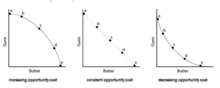
shape of PPC
- constant opportunity cost:
- increasing opportunity cost:
tutorial video 1
production possibilities curve as a model of a country's economy
tutorial video 2
PPCs for increasing, decreasing and constant opportunity cost
tutorial video 3
opportunity cost and comparative advantage using a PPC and an output table
Chapter 6: Classification of goods and services
- free good
- private good
- rivalry
- excludability
- public good
- non-excludability
- non-rivalry
- free rider
Chapter 6: Classification of goods and services
- government expenditure
- non-rejectability
- merit good
- information failure
- market imperfection
- market failure
- demerit good
learning objectives
- meaning of:
- free goods and private goods
- public goods
- merit goods and demerit goods
- imperfect information in the market
excludability
- a good is excludable ...
- ... if other consumers can be prevented ...
- ... from using or consuming it.

rivalry
- a good is rival ...
- ... if only one person can consume it ...
- ... and therefore the good is not available for other consumers

non-rival good
- a good is non-rival ...
- ... when the amount available to others ...
- ... does not diminish.

determining the type of good
| excludable | non-excludable | |
|---|---|---|
| rival | private good | quasi-public good |
| non-rival | quasi-public good | public good |
private good
- private goods are bought and consumed ...
- ... by individual consumers or firms ...
- ... for their own benefit.
- private goods have two characteristics:
- excludability (i.e. by charging a price)
- rivalry (reduces availability)
free good
- goods that have zero opportunity cost ...
- ... since consumption is not limited by scarcity.

public good
- goods that have two characteristics ...
- non-excludable
- non-rival

quasi-public good
- goods that have two characteristics ...
- excludable
- non-rival

merit goods
- a good that is thought to be desirable ...
- ... but which is underprovided by the market.

demerit goods
- a good that is thought to be undesirable ...
- ... but which is overprovided by the market.

Positive externalities and public goods
Introduction to public good (Voyager and NASA)Part 2: The price system and the microeconomy
- Demand and supply curves
- Price elasticity, income elasticity and cross elasticity of demand
- Price elasticity of supply
- The interaction of demand and supply
- Consumer and producer surplus
Chapter 7: Demand and supply curves
- price mechanism
- consumers
- market
- demand
- supply
- supply chain
- notional demand
- effective demand
- demand curve (D)
- market demand
Chapter 7: Demand and supply curves
- demand schedule
- movement along a demand curve
- normal goods
- inferior goods
- substitute
- complement
- joint demand
- supply curve (S)
- supply schedule
- subsidies
Chapter 7: Demand and supply curves
- indirect tax
- extension of demand or supply
- contraction of demand or supply
Chapter 7: Demand and supply curves
- effective demand
- demand
- law of demand
- demand curve
- demand schedule
- derived demand
- supply curve
- supply schedule
- change in quantity demanded
- extension in demand
Chapter 7: Demand and supply curves
- contraction in demand
- change in quantity supplied
- extension in supply
- contraction in supply
- change in demand
- composite demand
- normal good
- inferior good
- indirect taxes
- subsidy
price mechanism
- the means of allocating resources ...
- ... in a market economy
consumers
- individuals or households ...
- ... who buy goods and services ...
- ... for their own use or for others
market
- where buyers and sellers ...
- ... get together to trade
demand
- the quantity of a product ...
- ... that consumers are willing and able ...
- ... to buy at different prices ...
- ... per period of time ...
- ... other things equal, ceteris paribus
supply
- the quantity of a product ...
- ... that producers are willing and able ...
- ... to sell at different prices ...
- ... within a time period ...
- ... other things equal, ceteris paribus
supply chain
- all the stages of a product's progress ...
- ... from raw materials, production ...
- ... and distributions ...
- ... until it reaches the consumer
notional demand
- where buyers may want to buy a product ...
- ... but which is not always backed up ...
- ... by the ability to pay
effective demand
- demand that is supported ...
- ... the ability to pay
demand curve (D)
- a line plotted on a graph ...
- ... that represents the relationship between ...
- ... the quantity demanded ...
- ... and the price of a product
market demand
- the total amount demanded ...
- ... by consumers
demand schedule
- the data from which ...
- ... a demand curve is drawn on a graph
movement along a demand curve
- shows how quantity demanded ...
- ... responds to a change in price
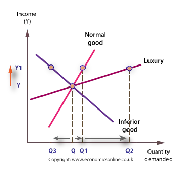
normal goods
- where the quantity demanded ...
- ... increases as income increases
inferior goods
- where the quantity demanded ...
- ... increases as income decreases
substitute
- an alternative good
complement
- a good consumed with another
joint demand
- when two goods ...
- ... are consumed together
supply curve (S)
- a line plotted on a graph ...
- ... that represents the relationship ...
- ... between the quantity supplied ...
- ... and the price of the product
supply schedule
- the data from which ...
- ... a supply curve is drawn on a graph
subsidies
- direct payments ...
- ... made by governments ...
- ... to producers of goods and services
indirect tax
- a tax levied ...
- ... on goods and services ...
- ... such as a general sales tax
extension of demand or supply
- an increase in the ...
- ... quantity demanded ...
- ... or quantity supplied
contraction of demand or supply
- a decrease in the ...
- ... quantity demanded ...
- ... or quantity supplied
price mechanism
- the means of allocating resources ...
- ... in a market economy
consumers
- individuals or households ...
- ... who buy goods and services ...
- ... for their own use or for others
market
- where buyers and sellers ...
- ... get together to trade
demand
- the quantity of a product ...
- ... that consumers are willing and able to buy ...
- ... at different prices per period of time ...
- ... other things equal, ceteris paribus
supply
- the quantity of a product ...
- ... that producers are willing and able to sell ...
- ... at different prices per period of time ...
- ... other things equal, ceteris paribus
supply chain
- all the stages of product's progress ...
- ... from raw materials, production and distribution ...
- ... until it reaches the consumer

notional demand
- where buyers may want to buy a product ...
- ... but which is not always backed up by the ability to pay
effective demand
- demand that is supported by the ability to pay
demand curve (D)
- a line plotted on a graph ...
- ... that represents the relationship between ...
- ... the quantity demanded and the price of a product
market demand
- total amount demanded by consumers
demand schedule
- data from which a demand curve is drawn on a graph

normal goods
- where the quantity demanded increases ...
- ... as income increases
inferior goods
- where the quantity demanded increases ...
- ... as income decreases

normal and inferior goods
inferior goods
substitute goods
- an alternative good

complement goods
- a good consumed with another

supply curve (S)
- a line plotted on a graph ...
- ... that represents the relationship between ...
- ... the quantity supplied and the price of the product.
supply schedule
- the data from which ...
- ... a supply curve is drawn on a graph
subsidies
- direct payments made by governments ...
- ... to producres of goods and services
indirect tax
- a tax levied on goods and services, ...
- ... such as a general sales tax
A Choice between Consumption Goods
How a Change in Income Affects Consumption Choices
How a Change in Price Affects Consumption Choices
The Foundations of a Demand Curve
|
|
An Example of Housing (a) As the price increases from P0 to P1 to P2 to P3, the budget constraint on the upper part of the diagram rotates clockwise. The utility-maximizing choice changes from M0 to M1 to M2 to M3. As a result, the quantity demanded of housing shifts from Q0 to Q1 to Q2 to Q3, ceteris paribus. (b) The demand curve graphs each combination of the price of housing and the quantity of housing demanded, ceteris paribus. The quantities of housing are the same at the points on both (a) and (b). Thus, the original price of housing (P0) and the original quantity of housing (Q0) appear on the demand curve as point E0. The higher price of housing (P1) and the corresponding lower quantity demanded of housing (Q1) appear on the demand curve as point E1. |
Farmer’s Market
Credit: modification of "Old Farmers' Market" by NatalieMaynor/Flickr, CC BY 2.0
Weirdest Celebrity Items Sold At Auction
Britney Spears' Gum, Brad Pitt's Breath And More (Huffpost)A Demand Curve for Gasoline
A Supply Curve for Gasoline
Shifts in Demand: A Car Example
Demand Curve
Demand Curve with Income Increase
Demand Curve Shifted Right
Factors That Shift Demand Curves
(b) The same factors, if their direction is reversed, can cause a decrease in demand from D0 to D1.
Shifts in Supply
Supply Curve
Setting Prices
Increasing Costs Leads to Increasing Price
Supply Curve Shifts
Factors That Shift Supply Curves
(b) The same factors, if their direction is reversed, can cause a decrease in supply from S0 to S1.
videos and tutorial
supply, demand and market equilibrium(Khan Academy)
law of demand
market demand as the sum of individual demand
supply, demand and market equilibrium
Chapter 8: Price elasticity, income elasticity and cross elasticity of demand
- elasticity
- elastic
- inelastic
- price elasticity of demand (PED)
- price elastic
- price inelastic
- perfectly inelastic
- perfectly elastic
Chapter 8: Price elasticity, income elasticity and cross elasticity of demand
- unit elasticity
- income elasticity of demand (YED)
- necessity good
- superior good
- cross elasticity of demand (XED)
Chapter 8: Price elasticity, income elasticity and cross elasticity of demand
- price elasticity of demand
- income elasticity of demand
- cross elasticity of demand (or cross-price elasticity of demand)
- substitute goods
- complementary goods
- perfectly inelastic
Chapter 8: Price elasticity, income elasticity and cross elasticity of demand
- inelastic
- unitary elasticity
- elastic
- perfectly elastic
- total revenue
elasticity
- a numerical measure of responsiveness ...
- ... of one variable following ...
- ... a change in another variable ...
- ceteris paribus or other things equal
elastic
- where the relative change ...
- ... in the quantity demanded ...
- ... is greater than ...
- ... the change in price, income ...
- ... or the prices of substitutes ...
- ... and complements
inelastic
- where the relative change ...
- ... in the quantity demanded ...
- ... is less than ...
- ... the change in price, income ...
- ... or the prices of substitutes ...
- ... and complements
price elasticity of demand (PED)
- measures of the responsiveness ...
- ... of the quantity demanded ...
- ... for a product following ...
- ... a change in the price of the product
price elastic
- when the relative change ...
- ... in the quantity demanded ...
- ... is greater than ...
- ... the change in price of the product
price inelastic
- when the relative change ...
- ... in the quantity demanded ...
- ... is less than ...
- ... the change in price of the product
perfectly inelastic
- where a change in price ...
- ... has no effect on the quantity demanded
perfectly elastic
- where all that is produced ...
- ... is sold at a given price
unit elasticity
- where the change in price ...
- ... is relatively the same as ...
- ... the change in quantity demanded
income elasticity of demand (YED)
- measures the responsiveness ...
- ... of the quantity demanded ...
- ... for a product following ...
- ... a change in income
necessity good
- a type of normal good ...
- ... with a YED ...
- ... that is close to zero
superior good
- a good with ...
- ... a YED ...
- ... greater than 1
cross elasticity of demand (XED)
- measures the responsiveness ...
- ... of the quantity demanded ...
- ... for one product ...
- ... following a ...
- ... change in the price ...
- ... of another product
On-Demand Media Pricing
Credit: modification of “160906_FF_CreditCardAgreements” by kdiwavvou/Flickr, Public Domain
elasticity
- a numerical measure of responsiveness ...
- ... of one variable following a change in another variable ...
- ... ceteris paribus

elastic
- where the relative change ...
- ... in the quantity demanded is greater ...
- ... than the change in price, income ...
- ... or the prices of substitutes and complements .
inelastic
- where the relative change ...
- ... in the quantity demanded is less ...
- ... than the change in price, income ...
- ... or the prices of substitutes and complements .
price elasticity of demand (PED)
- measures of the responsiveness ...
- ... of the quantity demanded for a product ...
- ... following a change in the price of the product.
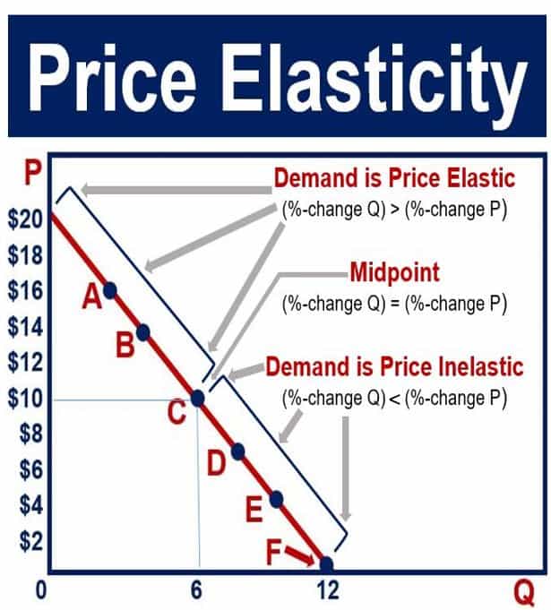
$PED = \frac{ \text{% change in quantity demanded} }{ \text{% change in price} }$
price elastic
- when the relative change in the quantity demanded ...
- ... is greater than ...
- ... change in price of the product.
price inelastic
- when the relative change in the quantity demanded ...
- ... is less than ...
- ... change in price of the product.
perfectly inelastic
- where a change in price ...
- ... has no effect ...
- ... on the quantity demanded
perfectly elastic
- where all that is produced ...
- ... is sold at ...
- ... a given price
unit elasticity
- where the change in price is ...
- ... relatively the same as ...
- ... the change in quantity demanded
price elasticity explained using a diagram
income elasticity of demand (YED)
- measures the responsiveness ...
- ... of the quantity demanded for a product ...
- ... following a change in income.
necessity good
- a type of normal good with a YED ...
- ... that is close to zero
superior good
- a good with a YED greater than 1
relationships between a change in income and quantity demanded
cross elasticity of demand (XED)
- measures the responsiveness of the ...
- ... quantity demanded ...
- ... for one product following ...
- ... a change in the price of another product.
$XED = \frac{ \text{% change in quantity demanded of product A} }{ \text{% change in the price of product B} }$

Calculating the Price Elasticity of Demand
Four part question (1/3)
- Define price elasticity of demand and explain how it is calculated. Provide two hypothetical examples of luxury goods, one with elastic demand and one with inelastic demand. Justify your classification for each example.
- Suppose the government imposes a significant tax increase on luxury cars to generate revenue. Analyze how this tax increase is likely to affect the price, quantity demanded, and total revenue in the luxury car market. Support your analysis with the appropriate elasticity concept.
Four part question (2/3)
- Calculate income elasticity for luxury cars if, over a year, the average income in the country increased by 10%, and the quantity demanded of luxury cars increased by 15%.
- Additionally, calculate the cross elasticity of demand between luxury cars and economy cars if the price of economy cars increased by 8%, and the quantity demanded of luxury cars decreased by 12%.
Four part question (3/3)
- Discuss the implications of the calculated income and cross elasticities for luxury car manufacturers. What do these elasticities reveal about the nature of luxury cars as normal or inferior goods and their relationship with economy cars?
- Provide recommendations for luxury car manufacturers based on your analysis.
Chapter 9: Price elasticity of supply
- price elasticity of supply
- price elastic supply
- price inelastic supply
- stocks
- perishability
price elasticity of supply (PES)
- a numerical measure ...
- ... of the responsiveness of the quantity supplied ...
- ... to a change in the price of the product
$PES = \frac{ \text{% change in quantity supplied} }{ \text{% change in price} }$
price elastic supply
- the quantity supplied ...
- ... responds more than proportionately ...
- ... to a change in its price
price inelastic supply
- the quantity supplied ...
- ... responds less than proportionately ...
- ... to a change in its price
factors affecting price elasticity supply
- number of producers
- amount of stocks
- time period
- existence of spare capacity
- length of the production period
- degree of factor mobility
Price Elasticity of Supply
Infinite Elasticity
Zero Elasticity
A Constant Unitary Elasticity Demand Curve
A Constant Unitary Elasticity Supply Curve
Passing along Cost Savings to Consumers
Passing along Higher Costs to Consumers
Elasticity and Tax Incidence
Elasticity and Tax Incidence
How a Shift in Supply Can Affect Price or Quantity
How a Shift in Supply Can Affect Price or Quantity
Chapter 10: The interaction of demand and supply
- equilibrium
- disequilibrium
- equilibrium price
- equilibrium quantity
- joint demand
- alternative demand
- derived demand
Chapter 10: The interaction of demand and supply
- joint supply
- rationing
- signalling
- price mechanism
- transmission of preferences
- incentivisation
- scarcity and choice
Demand and Supply Curves

Fall in supply

Good Weather for Salmon Fishing: The Four-Step Process
The Print News Market: A Four-Step Analysis
Higher Compensation for Postal Workers
Combined Effect of Decreased Demand and Decreased Supply
Shifts of Demand or Supply versus Movements along a Demand or Supply Curve
Demand and Supply Curves
Demand and Supply Curves
The figure displays a generic demand and supply curve.
Demand and Supply Curves
The horizontal axis shows the different measures of quantity: a quantity of a good or service, a quantity of labor for a given job, or a quantity of financial capital.
Demand and Supply Curves
The vertical axis shows a measure of price: the price of a good or service, the wage in the labor market, or the rate of return (like the interest rate) in the financial market.
Demand and Supply Curves
We can use the demand and supply curves to explain how economic events will cause changes in prices, wages, and rates of return.
Impact of Increasing Demand for Nurses 2020–2030
In 2020, the median salary for nurses was 75,330 USD. As demand for services increases, the demand curve shifts to the right (from $D_0$ to $D_1$) and the equilibrium quantity of nurses increases from $Qe_0$ to $Qe_1$. The equilibrium salary increases from $Pe_0$ to $Pe_1$.
Impact of Decreasing Supply of Nurses between 2020 and 2030
The increase in demand for nurses shown in the figure leads to both higher prices and higher quantities demanded. As nurses retire from the work force, the supply of nurses decreases, causing a leftward shift in the supply curve and higher salaries for nurses at $Pe_2$. The net effect on the equilibrium quantity of nurses is uncertain, which in this representation is less than $Qe_1$, but more than the initial $Qe_0$.
The effect of a 30% salt tax

The initial equilibrium. Initially the market equilibrium is at point A. The price is $P^*$ and the quantity of salt sold is $Q^*$.
The effect of a 30% salt tax

A 30% tax. A 30% tax is imposed on suppliers. Their marginal costs are effectively 30% higher at each quantity. The supply curve shifts.
The effect of a 30% salt tax

The new equilibrium. The new equilibrium is at B. The price paid by consumers has risen to $P_1$ and the quantity has fallen to $Q_1$.
The effect of a 30% salt tax

The tax paid to the government. The price received by suppliers (after they have paid the tax) is $P_0$. The double-headed arrow shows the tax paid to the government on each unit of salt sold.
Chapter 11: Consumer and producer surplus
- consumer surplus
- producer surplus
consumer surplus
- the difference between ...
- ... the price ...
- ... a consumer is willing to pay for a product ...
- ... and its market price
producer surplus
- the difference between ...
- ... the price ...
- ... a producer is willing to accept ...
- ... and what is actually paid
Demand and Supply for Gasoline
Demand and Supply for Gasoline
The demand curve (D) and the supply curve (S) intersect at the equilibrium point E, with a price of 1.40 dollar and a quantity of 600. The equilibrium price is the only price where quantity demanded is equal to quantity supplied. At a price above equilibrium like 1.80 dollar, quantity supplied exceeds the quantity demanded, so there is excess supply. At a price below equilibrium such as 1.20 dollar, quantity demanded exceeds quantity supplied, so there is excess demand.
Consumer and Producer Surplus
Consumer and Producer Surplus
The somewhat triangular area labeled by F shows the area of consumer surplus, which shows that the equilibrium price in the market was less than what many of the consumers were willing to pay. Point J on the demand curve shows that, even at the price of 90 dollar, consumers would have been willing to purchase a quantity of 20 million. The somewhat triangular area labeled by G shows the area of producer surplus, which shows that the equilibrium price received in the market was more than what many of the producers were willing to accept for their products. For example, point K on the supply curve shows that at a price of 45 dollar, firms would have been willing to supply a quantity of 14 million.
Efficiency and Price Floors and Ceilings
Efficiency and Price Floors and Ceilings
(a) The original equilibrium price is 600 dollar with a quantity of 20,000. Consumer surplus is T + U, and producer surplus is V + W + X. A price ceiling is imposed at 400 dollar, so firms in the market now produce only a quantity of 15,000. As a result, the new consumer surplus is T + V, while the new producer surplus is X. (b) The original equilibrium is $8 at a quantity of 1,800. Consumer surplus is G + H + J, and producer surplus is I + K. A price floor is imposed at 12 dollar, which means that quantity demanded falls to 1,400. As a result, the new consumer surplus is G, and the new producer surplus is H + I.
The effect of a 30% salt tax
- Identify the consumer surplus and producer surplus
- before the introduction of the tax
- after the introduction of the tax
- Discuss how taxes affect both surpluses.
consumer surplus and producer surplus

Part 3: Government microeconomic intervention
- Reasons for government intervention in markets
- Methods and effects of government intervention in markets
- Addressing income and wealth inequality
Chapter 12: Reasons for government intervention in markets
- market failure
- how governments intervene in markets
- controlling prices in markets
Chapter 13: Methods and effects of government intervention in markets
- impact & incidence of specific indirect taxes
- impact & incidence of subsidies
- direct provision of goods & services
- maximum & minimum prices
- buffer stock schemes
- provision of information
Chapter 14: Addressing income and wealth inequality
- income and wealth
- measuring income and wealth inequality
- economic reasons for inequality of income and wealth
- policies to redistribute income and wealth
Chapter 12: Reasons for government intervention in markets
- market failure
market failure
- when the free market ...
- ... does not make the best use ...
- ... of scarce resources
how do governments intervene in markets
- non-provision of public goods
- free rider problem
- private sector lack of interest
- opportunity cost of funding public goods
- over consumption of demerit goods
- under consumption of merit goods
controlling prices in markets
- set maximum prices
- use rent controls
- set minimum prices for agricultural products
controlling prices in markets - maximum prices
controlling prices in markets - maximum prices
controlling prices in markets - minimum prices
A Price Ceiling Example—Rent Control
European Wheat Prices: A Price Floor Example
Chapter 13: Methods and effects of government intervention in markets
- incidence
- maximum price
- minimum price
- buffer stock scheme
Chapter 13: Methods and effects of government intervention in markets
- indirect tax
- excise duty
- impact of tax
- incidence of tax
- specific tax
- subsidy
- impact of a subsidy
Chapter 13: Methods and effects of government intervention in markets
- incidence of a subsidy
- direct provision of goods and services
- maximum price
- minimum price
- price stabilisation
- buffer stock
incidence
- the extent to which ...
- ... the tax burden is borne ...
- ... by the producer ...
- ... or the consumer or both
maximum price (or price ceiling)
- a price that is fixed.
- the market price ...
- ... must not exceed this price.
minimum price (price floor)
- a price that is fixed.
- the market price ...
- ... must not go below this price.
buffer stock scheme
- a type of commodity agreement ...
- ... designed to limit price fluctuations
types of indirect taxes
- ad valorem : proportion or percentage of the price
- specific taxes : fixed amount per unit purchased
impact of indirect tax
- goal : discourage production and consumption of demerit goods
- tax imposed on the producer ...
- ... but passed on to consumers
impact of taxation

impact of taxation

impact of taxation

impact of taxation
impact of taxation

incidence of an indirect tax
- extent to which the tax burden is ...
- ... borne by the producer, ...
- ... by the consumer ...
- ... or by both
incidence of an indirect tax depends on ...
... the price elasticity of demand for the product
- the more inelastic the PED
$\longrightarrow$ easier it is to pass tax to the consumer
$\longrightarrow$ essential products are highly taxed - the more elastic the PED
$\longrightarrow$ consumer buys less as price $\uparrow$
$\longrightarrow$ producer will absorb tax
impact and incidence of subsidies
- ...
- ...
Chapter 14: Addressing income and wealth inequality
- wealth
- Gini coefficient
- informal economy
- minimum wage
- transfer payment
- progressive tax
- inheritance tax
- capital tax
Chapter 14: Addressing income and wealth inequality
- income
- wealth
- Gini coefficient
- minimum wage
- transfer payment
wealth
- a stock of assets ...
- ... that has been built up over time
Gini coefficient
- a numerical measure ...
- of income inequality
informal economy
- the part of the economy ...
- ... that is not regulated, protected or taxed ...
- ... by the government
minimum wage (expressed as wage per hour)
- the least amount ...
- ... an employer can ...
- ... legally pay one of its workers
transfer payment
- a payment made by ...
- ... the government ...
- ... to certain members of the community ...
- ... who may be unable to work ...
- ... or are in need of assistance
progressive tax
- one where the rate of taxation ...
- ... rises more than proportionately ...
- ... to the rise in income
inheritance tax
- a progressive tax ...
- ... on an inheritance or gift
capital tax
- a progressive tax paid ...
- ... annually ...
- ... on the difference between ...
- ... the buying and the selling price ...
- ... of an asset
difference between income and wealth
- income : reward for the services of a factor of production
- wages, salaries, bonuses
- rent, interest, profits
- wealth : stock of assets that someone has built up over time
- businesses, property
- shares, gold
- flow vs. stock
income $\longrightarrow$ flow concept
wealth $\longrightarrow$ stock concept
measuring income and wealth inequality
- Gini coefficient
- value $\longrightarrow$ 0 : equally distributed
- value $\longrightarrow$ 1 : inequality
economic reasons
for inequality of income & wealth
- no formal employment opportunities
- poor vocational training
- no investment in education & health sector
- poor infrastructure
- low rate of savings
- no access to loans
policies to redistribute income and wealth
- reduce income inequality
- redistribute wealth
$\longrightarrow$ dependent on tax revenues
policies to redistribute income and wealth
- minimum wage rates
- transfer payments
- taxation
- state provision of goods & services
minimum wage
- advantages
- reduces poverty
- disadvantages
- workers in informal sector are excluded
- self-employed workers are excluded
- critics say that it may create unemployment
- European countries by minimum wage
wage determination - minimum wage

transfer payment
- payment from tax revenue to vulnerable individuals
- examples
- pensions
- unemployment benefits
- housing allowances
- food coupons
- child benefits
- advantages vs. disadvantages
progressive tax
- high earners tax rate : 80%
- low earners tax rate : 20%-40%
- see real values for Luxembourg
$\longrightarrow$ reduces income differential
Part 4: The macroeconomy
- National income statistics
- Introduction to the circular flow of income
- Aggregate demand and aggregate supply analysis
- Economic growth
- Unemployment
- Price stability
Chapter 15: National income statistics
- national income
- gross domestic product (GDP)
- gross national income (GNI)
- net national income (NNI)
- at current market prices
- at constant prices
Chapter 15: National income statistics
- GDP deflator
- exports
- imports
- depreciation (of capital)
- net domestic product (NDP)
- net national product (NNP)
What is gross domestic product?
national income
- a country's total output
explore the national accounts data for Luxembourg (Statec)
national income statistics
- measures of the total output ...
- ... (income and expenditure) ...
- ... of an economy
gross domestic product (GDP)
- the total output ...
- ... produced in a country
gross domestic product (GDP)
Nominal gross domestic product (GDP) from OECD Real gross domestic product (GDP) from OECDgross national income (GNI)
- GDP ...
- ... plus net income ...
- ... from abroad
gross national income (GNI)
GNI data and definition (OECD)net property income from abroad
- receipts ...
- ... of profit, rent and interest ...
- ... earned on the ownership ...
- ... of foreign assets minus the payments ..
- ... of profit, rent and interest
- ... to non-residents
compensation of employees
- income of workers ...
- ... who work in another country ...
- ... for a short period of time
gross national disposable income
- GNI ...
- ... plus net transfers of workers' income ...
- ... to their relatives ...
- ... to and from other countries
multinational companies (MNCs)
- firms that operate ...
- ... in more than one country
circular flow of income
- a simplified view of ...
- ... how income flows ...
- ... around the economy

methods of measuring GDP
- output method
- income method
- expenditure method
output method
- a way of measuring GDP ...
- ... by calculating the total production ...
- ... of goods and services ...
- ... used in their production
value added
- the difference between ...
- ... the price at which products are sold ...
- ... and the price of goods and services ...
- ... used in their production
income method
- a way of measuring GDP ...
- ... by totalling all the incomes earned ...
- ... in producing the country's output
expenditure method
- a way of calculating GDP ...
- ... by totalling all the spending ...
- ... on the country's output
market prices
- prices paid ...
- ... by consumers ...
- ... that take into account ...
- ... indirect taxes and subsidies
basic prices
- prices charged by producers ...
- ... before the addition of indirect taxes ...
- ... and the deduction of subsidies
gross investment
- total spending on capital goods
net domestic product (NDP)
- GDP minus depreciation
net national income (NNI)
- gross national income (GNI) minus depreciation
net investment
- additions to the capital stock
depreciation (of capital goods)
- the value of capital goods ...
- ... that have worn out or become out-of-date
Chapter 16: Introduction to the circular flow of income
- circular flow of income
- closed economy
- open economy
- injection
- leakage (or withdrawal)
equilibrium income

Equilibrium point is where the savings line intersects with the investment line.
injection and leakage (or withdrawal)

Equilibrium income in a four-sector economy.
injection and leakage (or withdrawal)

At Y$_1$, we have leakages $>$ injections. Spending in the economy will decrease and therefore income will fall restoring the initial equilibrium.
injection and leakage (or withdrawal)

At Y$_2$, we have injections $>$ leakages. Spending in the economy will increase and therefore income will start rising restoring the initial equilibrium.
equilibrium income
The equality total investment $=$ total savings is essential for macroeconomic stability.
disequilibrium income

If savings exceed investment, it may indicate an excess of available funds, ... .
disequilibrium income
... which could lead to a decrease in interest rates or increased investment in the economy.
disequilibrium income
Excess saving and limited investment opportunities. There is an excess supply of funds in the financial markets ...
disequilibrium income
... borrowers are in a favourable position because lenders are competing to lend out their savings ...
disequilibrium income
... therefore lenders may be willing to accept lower interest rates.
disequilibrium income

In the context of lower interest rates, ...
disequilibrium income
... it becomes more attractive for borrowers to take out loans for investment projects.
Chapter 17: Aggregate demand and aggregate supply analysis
- aggregate demand (AD)
- aggregate supply (AS)
aggregate demand (AD)
- the total demand ...
- ... for an economy's goods and services ...
- ... at a given price level ...
- ... in a given time period
aggregate demand (AD)
$ \text{AD} = \text{C} + \text{I} + \text{G} + (\text{X}-\text{M}) $- $\text{C}$ : consumer expenditure
- $\text{I}$ : investment
- $\text{G}$ : government spending
- $\text{X}$ : exports of goods and services
- $\text{M}$ : imports of goods and services
consumer expenditure
- spending by households ...
- ... on goods and services
net exports
- exports minus imports
- $\text{NX} = \text{X} - \text{M}$
exchange rate
- the price ...
- ... of one currency ...
- ... in terms of ...
- ... another currency
aggregate supply (AS)
- the total output (real GDP) ...
- ... that producers in an economy ...
- ... are willing and able ...
- ... to supply ...
- ... at a given price level ...
- ... in a given time period
short-run aggregate supply (SRAS)
- the total output of an economy ...
- ... that will be supplied ...
- ... when there has not been enough time ...
- ... for the prices of factors of production ...
- ... to change
long-run aggregate supply (LRAS)
- the total output of a country ...
- ... supplied in the period ...
- ... when prices of factors of production ...
- ... have fully adjusted
average cost
- the cost ...
- ... per unit of output
supply-side shocks
- large and unexpected changes ...
- ... in short-run aggregate supply
Keynesians
- people who agree with the view of ...
- ... the economist John Maynard Keynes ...
- ... that government intervention ...
- ... is needed to achieve full employment

John Maynard Keynes (1883-1946)
new classical economist
- economists who think that ...
- ... the LRAS curve is vertical ...
- ... and that the economy will move towards ...
- ... full employment ...
- ... without government intervention
Keynesian Economics vs. Classic Economics
- Keynesian Economics
- increase consumer demand through government spending on:
- infrastructure
- unemployment benefits
- education
- government spending is necessary to maintain full employment
- Classic Economics
- promotes laissez-faire
- limit government intervention
- target firms not consumers
macroeconomic equilibrium
- the output and price level ...
- ... achieved where ...
- ... AD equals AS
aggregate demand and supply

Macroeconomic equilibrium: The point of equilibrium is where AD and AS intersect.
aggregate demand and supply

The Keynesian long-run aggregate supply curve.
aggregate demand and supply

The new classical long-run aggregate supply curve.
US economy : consumer price and interest rate
US economy : consumer price and interest rate
US economy : real GDP and interest rate
What happens to the interest rate right before recessions (grey area) and what happens during recessions?
US economy : tax revenues and real GDP
How do tax revenues change throughout the economic cycle?
US economy : tax rates and real GDP
How do tax rates change throughout the economic cycle?
Chapter 18: Economic growth
- economic development
- nominal (or money) GDP
- real GDP
- base year
- constant prices
- price index
- GDP deflator
- efficiency and inefficiency
- recession
- scarcity and choice
Chapter 18: Economic growth
- economic growth
- business cycle (or trade cycle)
- labour-intensive production
- capital-intensive production
Economic growth
economic development
- an increase ...
- ... in welfare and ...
- ... quality of life
nominal (or money) GDP
- total output ...
- ... measured in ...
- current prices
real GDP
- total output ...
- ... measured in ...
- ... constant prices
base year
- the reference point ...
- ... in time.
- it is the starting year ...
- ... in an index and ...
- ... is given a value of 100
constant prices (real prices)
- prices ...
- in a base year
current prices (nominal prices)
- prices ...
- indicated at ...
- ... a given moment in time
price index
- a way of comparing ...
- ... changes in the price level ...
- ... over time.
- the value of the first year ...
- ... in the index (base year) ...
- ... is set at 100 and ...
- ... the value of each following year ...
- ... is a percentage of it.
GDP deflator
- the price index ...
- ... of all domestically produced ...
- ... goods and services.
efficiency and inefficiency
- when an economy ...
- ... is producing ...
- ... inside its PPC, ...
- ... it is inefficiency
recession
- a decline in ...
- ... real GDP ...
- ... over at least ...
- ... two consecutive quarters
GDP Growth Calculation
GDP Growth Rate is calculated by the percentage increase in GDP from one period to the next
\[ \text{GDP Growth Rate (%)} = \left( \frac{\text{GDP}_{\text{current period}} - \text{GDP}_{\text{previous period}}}{\text{GDP}_{\text{previous period}}} \right) \times 100 \]
productive capacity

Inefficieny point.
productive capacity

Increase in productive capacity.
AD/AS diagram

AD and AS curve.
AD/AS diagram

Economic growth resulting from higher aggregate demand (AD).
AD/AS diagram

Economic growth resulting from higher aggregate supply (AS).
Chapter 19: Unemployment
- unemployment
- unemployment rate
- labour force
- working population
- dependency ratio
- participation rate
- claimant count
- labour force survey
Unemployment rate
Labor market
Credit: modification of "Hospital do Subúrbio" by Jaques Wagner Governador/Flickr Creative Commons, CC BY 2.0
Labor Market Example
Technology and Wages: Applying Demand and Supply
A Living Wage: Example of a Price Floor
labour force participation rate
- percentage of ...
- ... the total population of working age ...
- ... who are actually classified as ...
- ... being part of the labour force
level of unemployment
- total number of workers...
- ... who are unemployed
unemployment and employment
- employment rate is the ...
- proportion of the working age population ...
- ... who are in work ...
- ... and not ...
- ... the proportion of labour force in work.
$ \text{unemployment rate} + \text{employment rate} \neq 100\% $
stock vs. flow
- stock: measured at a particular time period
- flow: measured over a period of time period
methods of measuring unemployment
- claimant count measure:
count the registered unemployed (e.g. for benefits) - labour force survey measure:
survey-based by asking people
What are advantages and disadvantages of each method?
causes of unemployment
- frictional unemployment
- structural unemployment
- cyclical unemployment
frictional unemployment
- job-to-job search
- voluntary unemployment
- search unemployment
- casual unemployment
- seasonal unemployment
structural unemployment
- regional unemployment
- technological unemployment
- international unemployment
cyclical unemployment
- demand-deficient unemployment
- AD falls
consequences of unemployment
- workers: income $\downarrow$
- unemployed:
- duration uf unemployment makes it harder to find a new job
- decline in physical and mental health
- firms:
- not faced with wage rises
- lower demand for goods and services
Chapter 20: Price stability
- barter
- price stability
- inflation rate
- inflation
- price level
- creeping inflation
- hyperinflation
- deflation
- disinflation
Chapter 20: Price stability
- annual average method
- year-on-year method
- consumer price index (CPI)
- money values
- real data
- cost-push inflation
- wage-price spiral
- demand-pull inflation
- monetarists
Chapter 20: Price stability
- menu costs
- shoe leather costs
- fiscal drag
- inflationary noise
- total costs
- debtors
Chapter 20: Price stability
- inflation
- creeping inflation
- accelerating inflation
- hyperinflation
- deflation
- disinflation
- general price level
Chapter 20: Price stability
- cost of living
- consumer price index (CPI)
- sampling
- household expenditure
- weights
- base year
- nominal value
Chapter 20: Price stability
- real value
- demand-pull inflation
- monetary inflation
- cost-push inflation
- anticipated inflation
- unanticipated inflation
- imported inflation
Chapter 20: Price stability
- menu costs
- shoe lether costs
- fiscal drag
- stagflation
Inflation of consumer prices
Consumer price index
inflation
- a general increase ...
- ... in the average level of prices ...
- ... in an economy ...
- ... over a period of time
creeping inflation
- a situation where ...
- ... the rate of inflation ...
- ... is reasonably low ...
- ... say about 2%
accelerating inflation
- a situation where ...
- ... the rate of inflation ...
- ... is rising ...
- ... over a period of time
hyperinflation
- a situation where ...
- ... the rate of inflation ...
- ... is becoming very high ...
- ... and is damaging confidence ...
- ... in the country’s economy
deflation
- a general decrease ...
- ... in the average level of prices ...
- ... in an economy ...
- ... over a period of time
disinflation
- a general increase ...
- ... in the average level of prices ...
- ... in an economy ...
- ... over a period of time ...
- ... where the rate of increase ...
- ... is less than ...
- ... in the previous time period
general price level
- the average level of prices ...
- ... of all consumer goods and services ...
- ... in an economy ...
- ... at a given time
cost of living
- the cost of ...
- ... a selection of goods and services ...
- ... that are consumed by ...
- ... an average household ...
- ... in an economy ...
- ... at a given time
consumer price index (CPI)
- a way of measuring changes in the prices ...
- ... of a number of ...
- ... consumer goods and services ...
- ... in an economy ...
- ... over a period of time
sampling
- the use of a representative sample ...
- ... of goods and services ...
- ... consumed in an economy ...
- ... to give an indication of changes ...
- ... in the cost of living
household expenditure
- a survey is taken on ...
- ... a regular basis (usually every month) ...
- ... to record changes in the prices ...
- ... of a selection of goods and services ...
- ... that constitutes a representative basket
weights
- the items in a representative sample ...
- ... of goods and services ...
- ... bought by people in an economy ...
- ... will not all be of the same importance; ...
- weights are given ...
- ... to each of the items ...
- ... to reflect the relative importance ...
- ... of the different components in the basket ...
- ... and so a price index ...
- ... involves a weighted average
base year
- a year chosen so that comparisons ...
- ... can be made over a period of time;
- the base year for an index ...
- ... is given a value of 100
nominal value
- the value of a sum of money ...
- ... without taking into account ...
- ... the effects of inflation
real value
- the value of a sum of money ...
- ... after taking into account (removing) ...
- ... the effects of inflation
demand-pull inflation
- a rise in the ...
- ... general level of prices ...
- ... in an economy ...
- ... caused by too much demand ...
- ... for goods and services
causes of inflation
- cost-push inflation
- demand-pull inflation
consequences of inflation
- costs of inflation
- benefits of inflation
- factors affecting the consequences of inflation
- recent reductions in global inflation
consequences of inflation: costs of inflation
- $(X-M) \downarrow$
- unplanned redistribution of income
- menu costs
- shoe leather costs
- fiscal drag
- discouragement of investment
- inflationary noise
- inflation causing inflation
consequences of inflation: benefits of inflation
- output $\uparrow$
- burden of debt $\downarrow$
- some unemployment $\downarrow $ (pause wage rises)
consequences of inflation: factors affecting
- cause of inflation : demand-pull vs. cost-push
- rate of inflation : high vs. low
- rate of inflation : accelerating vs. stable
- expected vs. unexpected inflation rate
- relative inflation rate to other countries
consequences of inflation: recent reductions in global inflation
- advances in technology : costs $\downarrow$ $\longrightarrow$ AD $\uparrow$
- increased international competition
- changes in the labour market
Causes & consequences of deflation
deflation $\longrightarrow$ burden of debt $\uparrow$
$\longrightarrow$ real rate of interest $\uparrow$ $\longrightarrow$ menu cost
- good deflation : as a result of AS $\uparrow$
price level $\downarrow$ & real GDP $\uparrow$ - bad deflation : as a result of AD $\downarrow$
price level $\downarrow$ & real GDP $\downarrow$
[add diagram]
Extract: How should you fight inflation?
read How should you fight inflation?
by Joseph Stiglitz

aggregate demand and aggregate supply.
Video: Inflation (Bank of England)
Extract: Global Inflation
read Peak inflation? The new dilemma for central banks from FT
Part 5: Government macroeconomic intervention
- Government macroeconomic policy objectives
- Fiscal policy
- Monetary policy
- Supply-side policy
Chapter 21: Government macroeconomic policy objectives
- inflation target
- unemployment
- economic growth
Annual budget of NASA
Central government expenditure as share of GDP
Chapter 22: Fiscal policy
- fiscal policy
- government budget
- budget deficit
- budget surplus
- balanced budget
- national debt
Chapter 22: Fiscal policy
- direct tax
- income tax
- indirect tax
- specific tax
- ad valorem tax
- progressive taxation
Chapter 22: Fiscal policy
- regressive taxation
- proportional taxation
- flat-rate tax
- marginal tax rate
- average tax rate
- canons of taxation
Chapter 22: Fiscal policy
- capital spending (or investment spending)
- current spending
- discretionary fiscal policy
- automatic stabilisers
- expansionary fiscal policy
- contractionary fiscal policy
fiscal policy
- the use of ...
- ... taxation and government spending ...
- ... to influence aggregate demand
budget
- an annual statement ...
- ... in which the government ...
- ... outlines plans for its ...
- ... spending and tax revenue
budget surplus
- government revenue ...
- ... exceeding ...
- ... government expenditure
budget deficit
- government expenditure ...
- ... exceeding ...
- ... government revenue
balanced budget
- government revenue ...
- ... equalling ...
- ... government expenditure
automatic stabilisers
- changes in ...
- ... government spending and taxation ...
- ... that occur to ...
- ... reduce fluctuations ...
- ... in aggregate demand ...
- ... without any alteration ...
- ... in government policy
cyclical budget deficit
- a budget deficit ...
- ... caused by a decline ...
- ... in economic activity
structural budget deficit
- a budget deficit ...
- ... caused by an imbalance between ...
- ... government spending and taxation
tax base
- the coverage of ...
- ... what is taxed
national debt
- the total amount ...
- ... of government debt
specific taxes
- taxes that are charged ...
- ... as a set amount ...
- ... per unit
sin taxes
- taxes on products ...
- ... considered harmful to consumers
direct taxes
- taxes on ...
- ... income and wealth
tax avoidance
- the legal bending ...
- ... of the rules of the tax system ...
- ... to pay less tax
tax evasion
- the illegal non-payment ...
- ... or underpayment of a tax
regressive tax
- a tax which takes ...
- ... a larger percentage ...
- ... of the income or wealth ...
- ... of those on low incomes
proportional tax
- a tax which takes ...
- ... the same percentage ...
- ... of the income or wealth ...
- ... of all income groups
marginal rate of taxation (mrt)
- the proportion of ...
- ... extra income taken in tax
average rate of taxation (art)
- the proportion of income ...
- ... that is taxed
current government spending
- government spending ...
- ... on providing goods and services
capital government spending
- government spending ...
- ... on investment
exhaustive government spending
- government spending ...
- ... which makes use of resources
non-exhaustive government spending
- government spending ...
- ... which allows others to decide ...
- ... how resources are used
expansionary fiscal policy
- increases in ...
- ... government spending and ...
- ... cuts in taxes ...
- ... designed to increase aggregate demand
contractionary fiscal policy
- decreases in ...
- ... government spending and ...
- ... increases in taxes ...
- ... designed to reduce ...
- ... the growth of aggregate demand
discretionary fiscal policy
- deliberate changes in ...
- ... government spending and taxation
Chapter 23: Monetary policy
- monetary policy
- hot money
- quantitative easing
- open market operations
- expansionary monetary policy
- contractionary monetary policy
Chapter 24: Supply-side policy
- supply-side policy
- productivity
- productive capacity
- labour productivity
Part 6: International economic issues
- The reasons for international trade
- Protectionism
- Current account of the balance of payments
- Exchange rates
- Policies to correct imbalances in the current account of the balance of payments
Chapter 25: The reasons for international trade
- absolute advantage
- comparative advantage
- trading possibility curve
- bilateral trade
- multilateral trade
- globalisation
- specialisation
- free trade
- trade liberalisation
- trade creation
- World Trade Organization
- terms of trade
absolute advantage and comparative advantage
absolute advantage
- the ability to produce a good ...
- ... more efficiently (e.g. with less labour)
comparative advantage
- the ability to produce a good ...
- ... relatively more efficiently ...
- ... (i.e. at lower opportunity cost) ...
comparative advantage : example

comparative advantage : example

comparative advantage : example

comparative advantage : example

comparative advantage : example

comparative advantage : example

comparative advantage : example

comparative advantage : example

law of comparative advantage
- a theory arguing that there may be ...
- ... gains from trade arising ...
- ... when countries (or individuals) ...
- ... specialise in the production of goods ...
- ... or services in which they have ...
- ... a comparative advantage
trading possibilities curve
- shows the consumption possibilities ...
- ... under conditions of free trade
trade liberalisation
- a process of moving towards ...
- ... freer trade by ...
- ... removing restrictions on trade
terms of trade
- the ratio of ...
- ... export prices to ...
- ... import prices
income terms of trade
- the value of a ...
- ... country's exports ...
- ... divided by the ...
- ... price of its imports.
- measures the purchasing power ...
- ... of a country's exports in terms of ...
- ... the price of its imports
bilateral trade
- where trade takes place ...
- ... between two countries
multilateral trade
- where trade takes place ...
- ... between a number of countries
globalisation
- the process whereby there is ...
- ... an increasing world market ...
- ... in goods and services ...
- ... making an increase in multilateral trade ...
- ... more likely
specialisation
- the process whereby ...
- ... individuals, firms and economies ...
- ... concentrate on producing those products ...
- ... in which the have an advantage
free trade
- trade that is not restricted ...
- ... or limited ...
- ... by different types of ...
- ... import or export control
trade liberalisation
- the removal or reduction ...
- ... of restrictions or barriers ...
- ... to the free exchange of ...
- ... goods and services ...
- ... between countries
trade creation
- the creation of new trade ...
- ... as a result of ...
- ... the reduction or elimination ...
- ... of trade barriers
terms of trade
- the price of a ...
- ... country's exports in relation to ...
- ... the price of the country's imports
$$ \small\frac{ \text{index number showing the average price of exports} }{ \text{index number showing the average price of imports} } \times 100 $$
$\longrightarrow$ check data at OECD
$\longrightarrow$ check commodities TOT at IMF
causes of changes in the terms of trade
- demand for and supply of exports and imports
- inflation rate
- exchange rate
Prebisch-Singer hypothesis
- IED of manufactured goods
is far greater than
IED of primary products
- as income rises ...
- ... the demand for manufactured goods ...
- ... increase more than ...
- ... the demand for primary products
benefits of specialisation and free trade
- efficient allocation of resources
- factor endowment
- lower prices & better quality
- higher output
- economies of scale
- choice of products
- ...
- ... ...
- ... ...
- ... ...
- ...
Chapter 26: Protectionism
- protectionism
- tariff
- absolute poverty
- quota
- embargo
- voluntary export restraint
- exchange control
- infant industries
- dumping
- monopoly
- current account
Chapter 26: Protectionism
- absolute advantage
- protectionism
- tariff
- import duty
- quota
- export subsidy
- exchange controls
Chapter 26: Protectionism
- embargo
- voluntary export restraint (VER)
- infant industry argument
- sunrise industries
- sunset industries
- dumping
protectionism
- protecting domestic producers ...
- ... from foreign competition
tariff
- a tax imposed ...
- ... on imports
absolute poverty
- a condition where ...
- ... people's income ...
- ... is too low ...
- ... to enable them ...
- ... to meet their basic needs
quota
- a limit ...
- ... on imports
embargo
- a ban ...
- ... on imports and/or exports
voluntary export restraint
- a limit placed on imports ...
- ... reached with the agreement ...
- ... of the supplying country
exchange control
- restrictions on the purchases ...
- ... of foreign currency
infant industries
- new industries that have ...
- ... a low output ...
- ... and a high average cost
monopoly
- where one firm dominates the market ...
- ... due to having a large market share.
- A pure monopoly is a ...
- ... single seller with ...
- ... 100% market share
current account
- a record of the ...
- ... trade in goods, ...
- ... trade in services, ...
- ... primary income, ...
- ... and secondary income
protectionism
- measures taken by a country ...
- ... to restrict international trade
tariff
- a tax imposed on ...
- ... imported goods
quota
- an agreement by a country ...
- ... to limit its exports ...
- ... to another country ...
- ... to a given quantity
non-tariff barrier
- an obstacle to free trade ...
- ... other than a tariff
dumping
- where domestic producers ...
- ... face competition from imported goods ...
- ... that are priced ...
- ... below marginal cost, ...
- ... perhaps as a result of ...
- ... export subsidies
sunset industry
- an industry in decline ...
- ... that needs protection ...
- ... for its displaced workers
infant industry
- an industry that needs ...
- ... protection from international competition ...
- ... in the short run so that ...
- ... it can learn to become competitive
pro-free trade poster
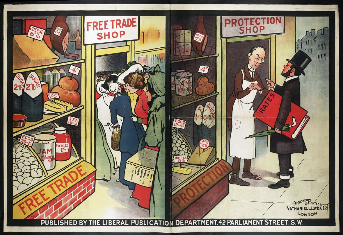
source: Wikipedia
anti-free trade poster

source: Wikipedia
tools of protection
- tariffs : taxes, usually on imports
- import quotas : limits on the quantity of imports
- export subsidies : subsidies given to exporters and domestic firms
- embargoes : a total ban on the imports of a particular product
- excessive administrative burdens (red tape)
impact of tariffs

a. market without trade
impact of tariffs

b. market with trade
impact of tariffs

c. market with trade : P $\downarrow$ and Q $\uparrow$
impact of tariffs

d. market with trade and after introduction of tariffs
Chapter 27: Current account of the balance of payments
- dividend payments
- exchange rate
- balance of payments account
- capital account
- financial account
- imbalance (in the current account of the balance of payments)
Chapter 27: Current account of the balance of payments
- current account deficit (of the balance of payments)
- current account surplus (of the balance of payments)
- balance (in the current account of the balance of payments)
Chapter 27: Current account of the balance of payments
- current account of the balance of payments
- balance of trade in goods account
- exports
- imports
- balance of trade in services account
- primary income
- net investment income
Chapter 27: Current account of the balance of payments
- secondary income
- current transfers
- deficit
- surplus
- external balance
- marginal propensity to import
The Balance Sheet
dividend payments
- a share of ...
- ... a firm's profits ...
- ... paid to its shareholders
exchange rate
- price of one currency ...
- ... in terms of another currency
balance of payments account
- a record of ...
- ... a country's economic transactions ...
- ... with the rest of the world ...
- ... over a year
capital account
- within the balance of payments, ...
- ... a record of the sale and purchase of ...
- ... copyrights, patents, trademarks, ...
- ... and money brought into the country ...
- ... by immigrants and taken out by emigrants
financial account
- within the balance of payments, ...
- ... a record of the transfer of ...
- ... financial and capital assets ...
- ... between the country ...
- ... and the rest of the world
imbalance
- debit items ...
- ... in the current account ...
- ... not equalling ...
- ... credit items
current account deficit
- the value of debit items ...
- ... on the current account ...
- ... exceeding ...
- ... the value of credit items
current account surplus
- the value of credit items ...
- ... on the current account ...
- ... exceeding ...
- ... the value of debit items
balance
- debit items ...
- ... on the current account ...
- ... equalling ...
- ... credit items
cumulative current account balance 1980-2008 (US$ billions)

source: Wikipedia
Chapter 28: Exchange rates
- floating exchange rate
- depreciation
- appreciation
- hot money flows
Chapter 28: Exchange rates
- exchange rate
- floating exchange rate
- depreciation
- appreciation
floating exchange rate
- an exchange rate ...
- ... that is determined ...
- ... by the market forces ...
- ... of demand and supply
depreciation
- a decrease ...
- ... in the international price ...
- ... of a currency ...
- ... caused by market forces
appreciation
- an increase ...
- ... in the international price ...
- ... of a currency ...
- ... caused by market forces
hot money flows
- flows of money ...
- ... moved around the world ...
- ... to take advantage of ...
- ... changes in interest rates ...
- ... and exchange rates
most traded currencies
.png/jcr:content/renditions/original-size.webp)
determination under floating exchange rate
- determined through market forces
- determined on the foreign exchange market
effect of an increase in the supply of currency

a. equilibrium value of the currency
effect of an increase in the supply of currency

b. supply of the currency in foreign exchange market increases
effect of an increase in the supply of currency

c. fall in the value of currency : depreciation
causes of changes in the floating exchange rate
- relative inflation rate $\downarrow$
- relative productivity $\uparrow$
- quality of products $\uparrow$
- incomes abroad $\uparrow$
$\uparrow$ value of exports $\rightarrow$ demand for currency $\uparrow$
causes of changes in the floating exchange rate
- foreigners demand for domestic shares
- demand for local currency to open accounts
$\rightarrow$ benefit from higher interest rates - short-term movements of money around the world $\rightarrow$ hot money flows
demand for currency $\uparrow$ $\rightarrow$ currency appreciates
interest rates and exchange rates
Chapter 29: Policies to correct imbalances in the current account of the balance of payments
- policy objective of stability
- fiscal policy
- monetary policy
- supply-side policy
- protectionist policy
essay-style questions (s23)
PPC, public good and merit good (s23_21)
- With the help of a diagram, explain the difference between the causes of a movement along, and a shift of, a production possibility curve (PPC) and consider which is likely to have the most immediate impact on an economy. [8 marks]
- Assess whether education should be classified as a public good rather than classified as a merit good. [12 marks]
cross-elasticity of demand and buffer stock scheme (s23_21)
- With the help of a formula, explain the meaning of cross elasticity of demand and consider which determinants are most important in establishing the size and sign of its coefficient. [8 marks]
- With the help of a diagram, assess whether the benefits of a buffer stock scheme for an agricultural product always outweigh its disadvantages. [12 marks]
AD/AS diagram, cost-push inflation, demand-pull inflation, monetary policy, supply-side policy and inflation (s23_21)
- With the help of an AD/AS diagram(s), explain cost-push inflation and demand-pull inflation in an economy and consider in what circumstances one may be more damaging than the other. [8 marks]
- Assess whether monetary policy or supply-side policy is likely to be more successful in reducing the rate of inflation in an economy. [12 marks]
depreciation, floating exchange rate, protectionism and international trade (s23_21)
- With the help of a diagram(s), explain the likely causes of a depreciation of a floating exchange rate and consider whether such a depreciation is always beneficial to an economy. [8 marks]
- Assess whether the arguments for protectionism in the context of international trade are always stronger than the arguments against. [12 marks]
consumer surplus, producer surplus, maximum price, transfer payments and low-income households (s23_22)
- With the help of a diagram(s), explain what is meant by consumer surplus and producer surplus and consider whether a rise in the price of a product because of higher costs of production is likely to always reduce the consumer surplus. [8 marks]
- A government wishes to keep the price of an essential food, such as rice, affordable to help
low-income households.
Assess whether a policy of fixing the maximum price for an essential food is likely to be more effective than a policy of making transfer payments to low-income households. [12 marks]
equilibrium price, equilibrium quantity, market equilibrium, wages, labour market, economic growth and entrepreneurship (s23_22)
- With the help of a diagram(s), explain what is meant by equilibrium in a market and consider the extent to which the equilibrium price and equilibrium quantity are likely to change for a product following an increase in the wages for labour across the whole economy. [8 marks]
- Entrepreneurs are vital in an economy to achieve long run economic growth.
Assess whether encouraging entrepreneurship or increasing another of the factors of production will be a more effective way to achieve long-run economic growth. [12 marks]
trade, absolute advantage, comparative advantage, protectionism, deficit in the current account, and balance of payments (s23_22)
- Two countries each produce two products and wish to trade with each other.
Explain the difference between the principles of absolute advantage and comparative advantage and consider whether the principle of comparative advantage is always the more important influence when each country is deciding whether to trade with each other. [8 marks] - Assess whether protectionism is the best way to correct a deficit in the current account of the balance of payments. [12 marks]
cost-push inflation, demand-pull inflation, depreciation, exchange-rate, and monetary policy (s23_22)
- Explain the difference between cost-push and demand-pull inflation and consider which is more likely to occur if there is a depreciation in the exchange rate of a country with few natural resources. [8 marks]
- Assess whether monetary policy is the only way to control a high rate of inflation. [12 marks]
income elasticity of demand, classification of goods, consumer surplus, and price elasticity of demand (s23_23)
- Explain, with the help of examples, the significance of the size and sign of the coefficient of income elasticity of demand for the classification of a good and consider how confident you are of this classification. [8 marks]
- When the price of a product changes, it usually changes the consumer surplus in the market.
Assess how variations in price elasticity of demand for a product determine the extent of changes in consumer surplus in a market. [12 marks]
government intervention, merit goods, and buffer stock schemes (s23_23)
- Explain why government intervention may be required to provide merit goods and consider why such intervention may not always be successful. [8 marks]
- Assess the effectiveness of government intervention through buffer stock schemes in agricultural markets. [12 marks]
circular flow of income, open economy, budget deficit, trade deficit, and investment in infrastructure (s23_23)
- With the help of a circular flow of income diagram, explain how equilibrium is determined in an open economy and consider whether a budget deficit or a trade deficit is more likely to cause lasting disequilibrium. [8 marks]
- Assess whether an increase in investment in new infrastructure projects will always have a positive impact on the circular flow of income in an economy. [12 marks]
monetary policy, inflation rate, macroeconomic objectives, and macroeconomic intervention (s23_23)
- Explain how monetary policy may be able to reduce the rate of inflation in an economy and consider the likely success of this policy. [8 marks]
- Assess how governments use macroeconomic intervention to achieve their macroeconomic objectives. [12 marks]
case study (s23)
Unemployment in India (extract and s23_21)
- Using the data in Fig. 1.1, calculate the change in India's unemployment rate between July 2020 and May 2021. [2 marks]
- Using the information provided, explain how agriculture caused seasonal unemployment in India in December 2020. [2 marks]
- Consider the extent to which difficulties may arise in the measurement of unemployment in India. [4 marks]
- Assess whether seasonal unemployment is likely to be a more serious problem than frictional unemployment for India's economy. [6 marks]
- Assess the possible measures that could be taken to increase employment in a country such as India. [6 marks]
Is Nigeria being held back by its dependence on oil and gas? (extract and s23_22)
- Compare the government budget balance of Nigeria in 2016 with the government budget balance in 2020. [2 marks]
- Using a production possibility curve (PPC) diagram, demonstrate the impact of the rising level of unemployment on the Nigerian economy. [2 marks]
- Consider the extent to which the removal of fuel subsidies in Nigeria would lead to an increase in inflation. [4 marks]
- Assess whether using supply-side policy is the best way to diversify the Nigerian economy away from its dependence on oil and natural gas exports. [6 marks]
- Assess whether adjusting the collection of direct tax or indirect tax is likely to be more effective in increasing the tax revenue collected by the Nigerian government. [6 marks]
Are doughnuts demerit goods? (extract and s23_23)
- Using the data in Fig. 1.1, calculate the percentage change in the value of sales of doughnuts in the US from 2011 to 2019. [2 marks]
- Explain one reason why the US market for doughnuts contracted in 2020. [2 marks]
- Comment on whether the demand for doughnuts in the US is income elastic or income inelastic. [2 marks]
- Explain why a doughnut might be regarded as a demerit good. [2 marks]
- With the help of a diagram, assess how the market for sugary foods in the UK might be affected by a ban on online advertising. [6 marks]
- Assess the likely effects on UK consumers and the UK government of a ban on online adverts for sugary foods. [6 marks]
case study (s22)
Inflation in Bangladesh (extract and s22_21)
- Describe the trend in the annual inflation rate of Bangladesh between 2009 and 2019. [2 marks]
- Explain why price changes in the food and the non-food sectors in Bangladesh are treated differently when calculating the CPI. [2 marks]
- Explain one domestic consequence and one external consequence for Bangladesh of having 'a relatively high rate of inflation'. [4 marks]
- Analyse, with the help of aggregate demand and aggregate supply diagrams, how increasing wages can cause both demand-pull and cost-push inflation in Bangladesh. [6 marks]
- 'However, there is always the possibility that tough monetary policies could do more harm
than good to an economy, compared with the possible use of fiscal policy.'
Discuss whether monetary policy or fiscal policy is more likely to be effective in controlling inflation. [6 marks]
Economic growth in Russia has slowed to well below the global average (extract and s22_22 and original article )
- Using Fig. 1.1
- Compare the rate of inflation in Russia in March 2015 with that in March 2020. [1 mark]
- What has happened to the price level over this period? [1 mark]
- Explain what could have caused real wages in Russia to decline between 2016 and 2018. [2 marks]
- Explain whether school lunches provided free-of-charge by the Russian government would be classified as private goods or public goods. [4 marks]
- Assess, using aggregate demand and aggregate supply analysis, the likely impact of the changes shown in Table 1.1 upon the rate of inflation in Russia. [6 marks]
- Discuss whether the 'huge decrease in the price of oil' and the fall in the value of the rouble might bring more opportunities than threats to the Russian economy. [6 marks]
The changing market for avocados (extract and s22_23)
- Describe the change in the level and source countries of the US’s imports of avocados from 2013 to 2018. [2 marks]
-
- Calculate the percentage change in the wholesale price of Mexican avocados between April 2019 and the end of July 2019. [1 marks]
- Explain one possible demand reason and one possible supply reason for this change in price. [4 marks]
- Using the information provided, consider whether the supply of avocados is price elastic or price inelastic in the short run and in the long run. [4 marks]
- Explain, with the help of a production possibility curve diagram, the opportunity cost to a New Zealand farmer of converting from dairy to avocado production. [3 marks]
- Discuss whether the price mechanism in the avocado market is working to allocate resources successfully. [6 marks]
general tips for your exam (2iec)
general tips for essay writing
- ensure that you offer a clear judgement that answers the question.
- draw upon your wide-ranging knowledge of economic concepts and terms to provide a coherent chain of reasoning.
- avoid narrow responses or superficial answers by practising going beyond two stage chains of reasoning
- ensure you are evaluating what you have written in the context of the question set.
- make effective use of a knowledge organiser so that your knowledge and understanding is precise.
- spend time planning your essay response in terms of the key points and evaluation that you want to make to avoid the risk of repetition
- ensure that examples given link tightly to the economic concept you are trying to address
- remember a judgement is expected to get the very top marks for evaluation
- plan out your answer - feeling your way through an answer risks an overlong first paragraph which lacks a precise understanding of the key concept
general tips for case studies
- whilst it is good to spend time on case studies looking at a specific firm, market or industry, it is essential that the focus is on showing an ability to link knowledge and understanding in context using appropriate examples
- start with the key concepts and see how they are applied to the case study you are looking at
- try to apply yourself to the context of the question - imagine yourself problem solving as an economist : contexts are often chosen that are relatable to you
general tips for short answers
- ensure you have mastered key knowledge of economic terms and concepts to avoid generic responses
- making effective use of supply and demand diagrams can help lock in knowledge and analysis marks or may provide a way into evaluation.
- make effective use of the data
- for calculate questions, numerical responses are the most simplest expected answer - it is important to show your workings to secure marks in case your final answer is incorrect
- for short 2 mark explain questions, an example will often help in securing a second mark
- fully label externalities diagrams.
- draw diagrams clearly and large enough for ease of interpretation
- for shifts in supply and demand consider the non-price determinants as identified in the data. Do not confuse shifts in supply with extensions in supply.
Rise in unemployment in period march 2023 to april 2024
*see* NotebookPart 7: The price system and the microeconomy
- Utility
- Indifference curves and budget lines
- Efficiency and market failure
- Private costs and benefits, externalities and social costs and benefits
- Types of cost, revenue and profit, short-run and long-run production
- Different market structures
- Growth and survival of firms
- Differing objectives and policies of firms
Chapter 30: Utility
- utility
- law of diminishing marginal utility
- total utility
- marginal utility
- equi-marginal principle
- individual demand curve
utility
- the satisfaction ...
- ... received from ...
- ... consumption

law of diminishing marginal utility
- as consumption increase, ...
- ... the satisfaction from consumption ...
- ... decreases
total utility
- the total satisfaction ...
- ... received from ...
- ... consumption
marginal utility
- the utility ...
- ... derived from the ...
- ... consumption of ...
- ... one more unit of ...
- ... the good or service
total utility and marginal utility
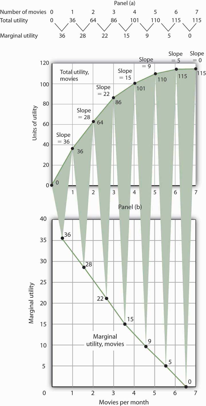
equi-marginal principle
- consumers ...
- ... maximise their utility ...
- ... where their marginal valuation ...
- ... for each product consumed ...
- ... is the same
$ \frac{MU_A}{P_A} = \frac{MU_B}{P_B} = \frac{MU_C}{P_C} = \ldots \frac{MU_N}{P_N} $
consequences of equi-marginal principle
$ \frac{MU_A}{P_A} = \frac{MU_B}{P_B} = \frac{MU_C}{P_C} = \ldots \frac{MU_N}{P_N} $
- total utility cannot be increased
- consumer equilibrium is achieved
- equi-marginal principle based on following assumptions :
- consumers have limited incomes
- consumers behave in a rational manner
- consumers seek to maximize utility
illustration of equi-marginal principle
$ \frac{MU_A}{P_A} = \frac{MU_B}{P_B} = \frac{MU_C}{P_C} = \ldots \frac{MU_N}{P_N} $
| product x ($1/pc) | product y ($2/pc) | |||
|---|---|---|---|---|
| MU | MU/P | quantity | MU | MU/P |
| 60 | 60 | 1 | 42 | 21 |
| 40 | 40 | 2 | 32 | 16 |
| 25 | 25 | 3 | 24 | 12 |
| 12 | 12 | 4 | 18 | 9 |
| 5 | 5 | 5 | 14 | 7 |
| 2 | 2 | 6 | 12 | 6 |
illustration of equi-marginal principle
$ \frac{MU_x}{P_x} = \frac{MU_y}{P_y} $
| product x ($1/pc) | product y ($2/pc) | |||
|---|---|---|---|---|
| MU | MU/P | quantity | MU | MU/P |
| 60 | 60 | 1 | 42 | 21 |
| 40 | 40 | 2 | 32 | 16 |
| 25 | 25 | 3 | 24 | 12 |
| 12 | 12 |
4 | 18 | 9 |
| 5 | 5 | 5 | 14 | 7 |
| 2 | 2 | 6 | 12 | 6 |
illustration of equi-marginal principle
$ \frac{MU_x}{P_x} = \frac{MU_y}{P_y} $
- consumer equilibrium is achieved where
- 4 units of x, and
- 3 units of y
- total utility score
$\underbrace{(60+40+25+12)}_{\text{sum of } MU_x} + \underbrace{(42+32+24)}_{ \text{sum of } MU_y } = 235$
how to calculate the total utility score
The total utility is equal to the sum of utilities gained from each unit of consumption.In the previous table, each unit of consumption is expected to have slightly less utility as more units are consumed.
derivation of individual demand curve from a given consumer equilibrium
| product x ($1/pc) | product y ($2/pc) | |||
|---|---|---|---|---|
| MU | MU/P | quantity | MU | MU/P |
| 60 | 60 | 1 | 42 | 21 |
| 40 | 40 | 2 | 32 | 16 |
| 25 | 25 | 3 | 24 | 12 |
| 12 | 12 | 4 | 18 | 9 |
| 5 | 5 | 5 | 14 | 7 |
| 2 | 2 | 6 | 12 | 6 |
derivation of individual demand curve from a given consumer equilibrium
| product x ($1/pc) | product y ($1/pc) | |||
|---|---|---|---|---|
| MU | MU/P | quantity | MU | MU/P |
| 60 | 60 | 1 | 42 | ? |
| 40 | 40 | 2 | 32 | ? |
| 25 | 25 | 3 | 24 | ? |
| 12 | 12 | 4 | 18 | ? |
| 5 | 5 | 5 | 14 | ? |
| 2 | 2 | 6 | 12 | ? |
What is the new consumer equilibrium? (Fig 30.3)
derivation of individual demand curve from a given consumer equilibrium
| product x ($1/pc) | product y ($1/pc) | |||
|---|---|---|---|---|
| MU | MU/P | quantity | MU | MU/P |
| 60 | 60 | 1 | 42 | 42 |
| 40 | 40 | 2 | 32 | 32 |
| 25 | 25 | 3 | 24 | 24 |
| 12 | 12 | 4 | 18 | 18 |
| 5 | 5 | 5 | 14 | 14 |
| 2 | 2 | 6 | 12 | 12 |
What is the new consumer equilibrium? (Fig 30.3)
derivation of individual demand curve from a given consumer equilibrium

limitations of the marginal utility theory
this theory relies on the following assumptions
- consumers are capable of ranking their wants
- consumers are able to assign a value to the satisfaction
- consumers act in a rational way
Chapter 31: Indifference curves and budget lines
- indifference curves
- marginal rate of substitution
- budget line
- substitution effect
- income effect
- Giffen good
indifference curves
- this shows ...
- ... all of the ...
- ... combinations of two goods ...
- ... that give a consumer ...
- ... equal satisfaction
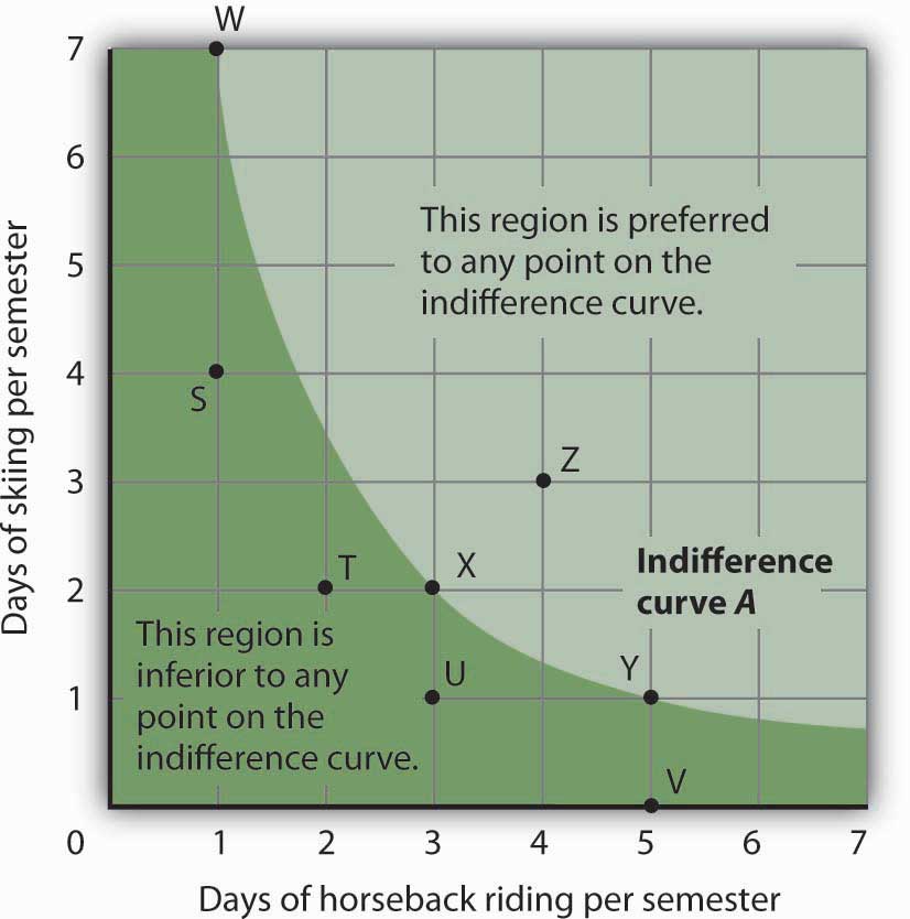
indifference curves
- this shows ...
- ... all of the ...
- ... combinations of two goods ...
- ... that give a consumer ...
- ... equal satisfaction
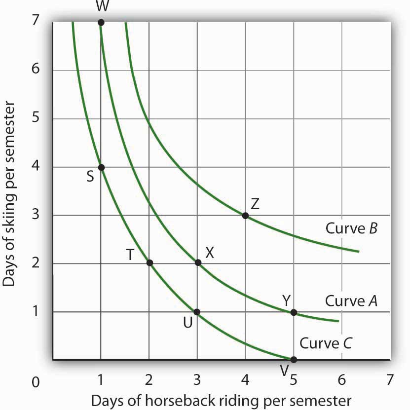
marginal rate of substitution
- the rate at which ...
- ... a consumer ...
- ... is willing to substitute ...
- ... one good for another
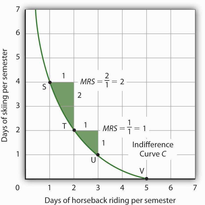
budget line
- the combinations of two goods ...
- ... that can be purchased ...
- ... with given income and ...
- ... given prices
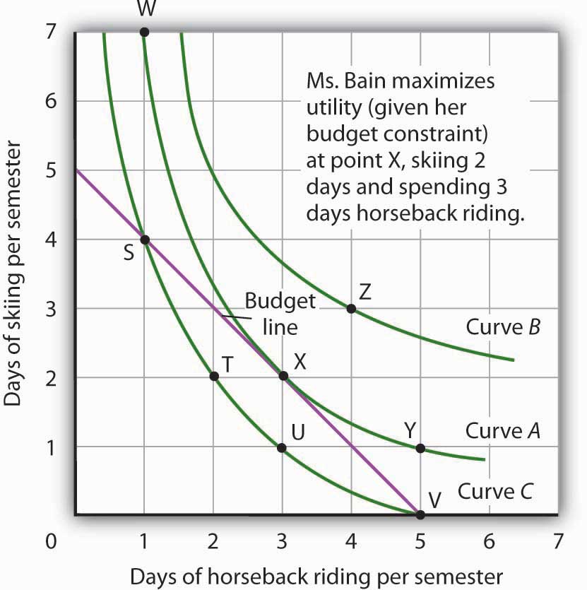
illustration: substitution effect
- apples (A) : 2€/kg
- oranges (O) : 1€/kg
- consumption so that the
utility-maximizing condition
holds for the two goods
$ \frac{MU_A}{2€} = \frac{MU_O}{1€} $
illustration: substitution effect
- apples (A) : 2€/kg $\rightarrow$ 1€/kg
- oranges (O) : 1€/kg
- $ \frac{MU_A}{1€} > \frac{MU_O}{1€} $ : disequilibrium
$\longrightarrow$ consumption of apples $\uparrow$
$\longrightarrow$ $MU_A$ $\downarrow$
illustration: substitution effect
- apples (A) : 2€/kg $\rightarrow$ 1€/kg
- oranges (O) : 1€/kg
- $ \frac{MU_A}{1€} > \frac{MU_O}{1€} $ : disequilibrium
$\longrightarrow$ consumption of oranges $\downarrow$
$\longrightarrow$ $MU_O$ $\uparrow$
substitution effect
- where, ...
- ... following a price change, ...
- ... a consumer will substitute ...
- ... the cheaper good for the one ...
- ... that is now relatively more expensive.
income effect
- where following a price change of a good, ...
- ... a consumer has higher real income and ...
- ... will purchase more of this good.
Giffen good
- a type of inferior good ...
- ... where the quantity demanded falls ...
- ... as price falls and ...
- ... the quantity demanded increases ...
- ... as price increases
effect of an increase in income on consumption of goods X and Y

effect of an increase in price of good X on consumption of goods X and Y

effect of an decrease in price of an inferior good X on consumption of goods X and Y

effect of an decrease in price of an Giffen good X on consumption of goods X and Y

Chapter 32: Efficiency and market failure
- economic efficiency
- productive efficiency
- allocative efficiency
- marginal cost
- Pareto optimality
- dynamic efficiency
economic efficiency
- where scarce resources ...
- ... are used in the most efficient way to ...
- ... produce maximum output
productive efficiency
- when a firm ...
- ... is producing at the ...
- ... lowest possible cost
allocative efficiency
- where price is equal to marginal cost;
- firms are producing those ...
- ... goods and services ...
- ... most wanted by consumers
marginal cost
- the addition to total cost ...
- ... when making one extra unit of output
$ MC = \frac{\Delta \text{total cost} }{ \Delta \text{quantity produced} } $
Pareto optimality
- where it is impossible to ...
- ... make someone better off without ...
- ... making someone else worse off
dynamic efficiency
- when resources are...
- ... allocated efficiently ...
- ... over time
market failure
- occurs whenever a free market ...
- ... fails to make the best use of ...
- ... scarce resources
market failure can be caused by :
- externalities
- merit and demerit goods
- public and quasi-public goods
- information failure
- adverse selection and moral hazard
- monopoly power
Chapter 33: Private costs and benefits, externalities and social costs and benefits
- externality
- third parties
- negative externality
- positive externality
- private costs (PC)
- private benefits (PB)
- external costs (EC)
- external benefits (EB)
- social costs (SC)
Chapter 33: Private costs and benefits, externalities and social costs and benefits
- social benefits (SB)
- deadweight welfare loss
- asymmetric information
- adverse selection
- moral hazard
- cost-benefit analysis
- shadow price
- benefit:cost ratio
externality
- where the actions of ...
- ... a producer or consumer ...
- ... give rise to side effects on others ...
- ... not directly involved in the action
third parties
- those not directly involved ...
- ... in the decision-making
negative externality
- where the side effects of an action ...
- ... have a negative impact that ...
- ... imposes costs on third parties
positive externality
- where the side effects of an action ...
- ... have a positive impact that ...
- ... provides benefits to third parties
private costs (PC)
- costs that are incurred ...
- ... by a consumer or by the firm ...
- ... that produces a good or service
private benefits (PB)
- benefits that accrue ...
- ... to the consumer or to the firm ...
- ... that produces a good or service
external costs (EC)
- costs incurred and paid for ...
- ... by a third party ...
- ... not involved in the action
external benefits (EB)
- benefits that are received ...
- ... by a third party ...
- ... not involved in the action
social costs (SC)
- the total costs ...
- ... of a particular action
social benefits (SB)
- total benefits ...
- ... of a particular action
deadweight welfare loss
- the loss in welfare ...
- ... arising from an inefficient ...
- ... allocation of resources
asymmetric information
- where one party ...
- ... has more or better information ...
- ... than another ...
- ... in a business transaction
adverse selection
- when sellers have information that ...
- ... buyers do not have on ...
- ... product quality or ...
- ... when buyers have information that ...
- ... sellers do not have ...
- ... on product quality
moral hazard
- the temptation to take risks ...
- ... when some other party ...
- ... is covering these risks
cost-benefit analysis
- a method of decision-making ...
- ... that takes into account ...
- ... the costs and benefits involved
shadow price
- one that is applied where ...
- ... there is no established ...
- ... market price available
benefit:cost ratio
- net benefits ...
- ... as a proportion of ...
- ... net costs
Chapter 34: Types of cost, revenue and profit, short-run and long-run production
- economies of scale
- isoquant
- total product
- production function
- marginal product
- law of diminishing returns
- average product
- profit maximisation
- fixed costs (FC)
Chapter 34: Types of cost, revenue and profit, short-run and long-run production
- variable costs (VC)
- increasing returns to scale
- decreasing returns to scale
- isocosts
- minimum efficient scale
- diseconomies of scale
- external economies of scale
- total revenue (TR)
Chapter 34: Types of cost, revenue and profit, short-run and long-run production
- average revenue (AR)
- marginal revenue (MR)
- price taker
- price maker
- profit
- normal profit
- supernormal profit
- subnormal profit
economies of scale
- the benefits gained from ...
- ... falling long-run average costs ...
- ... as the scale of output ...
- ... increases

isoquant
- a curve showing ...
- ... combinations of labour and capital ...
- ... to produce a given level of output
total product
- the same as total output
production function
- the maximum possible output from ...
- ... a given set of factor inputs

marginal product (MP)
- the change in output ...
- ... arising from the use of ...
- ... one more unit of a factor of production
$ MP = \frac{ \Delta \text{output} }{ \Delta \text{factor of production} }$
law of diminishing returns
or law of variable proportions
- where the output from ...
- ... an additional unit of input leads to ...
- ... a fall in the marginal product

average product
- total product divided by ...
- ... the number of workers employed.
- a simple measure of productivity
profit maximisation
- objective of a firm
- the difference between ...
- ... total revenue and ...
- ... total cost ...
- ... is at a maximum
fixed costs (FC)
- costs ...
- ... that are independent of output ...
- ... in the short run
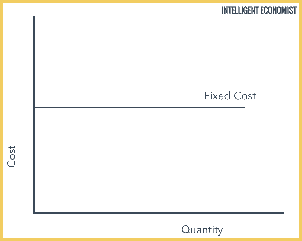
variable costs (VC)
- costs ...
- ... that vary directly with output ...
- ... in the short run

increasing returns to scale
- where output increases ...
- ... at a proportionately faster rate ...
- ... than the increase in factor inputs
decreasing returns to scale
- where factor inputs increase ...
- ... at a proportionately faster rate than ...
- ... the increase in output
isocosts
- lines of constant relative costs ...
- ... for factors of production

minimum efficient scale
- lowest level of output ...
- ... at which costs are minimised

diseconomies of scale
- where long-run average costs ...
- ... increase as the ...
- ... scale of output increases
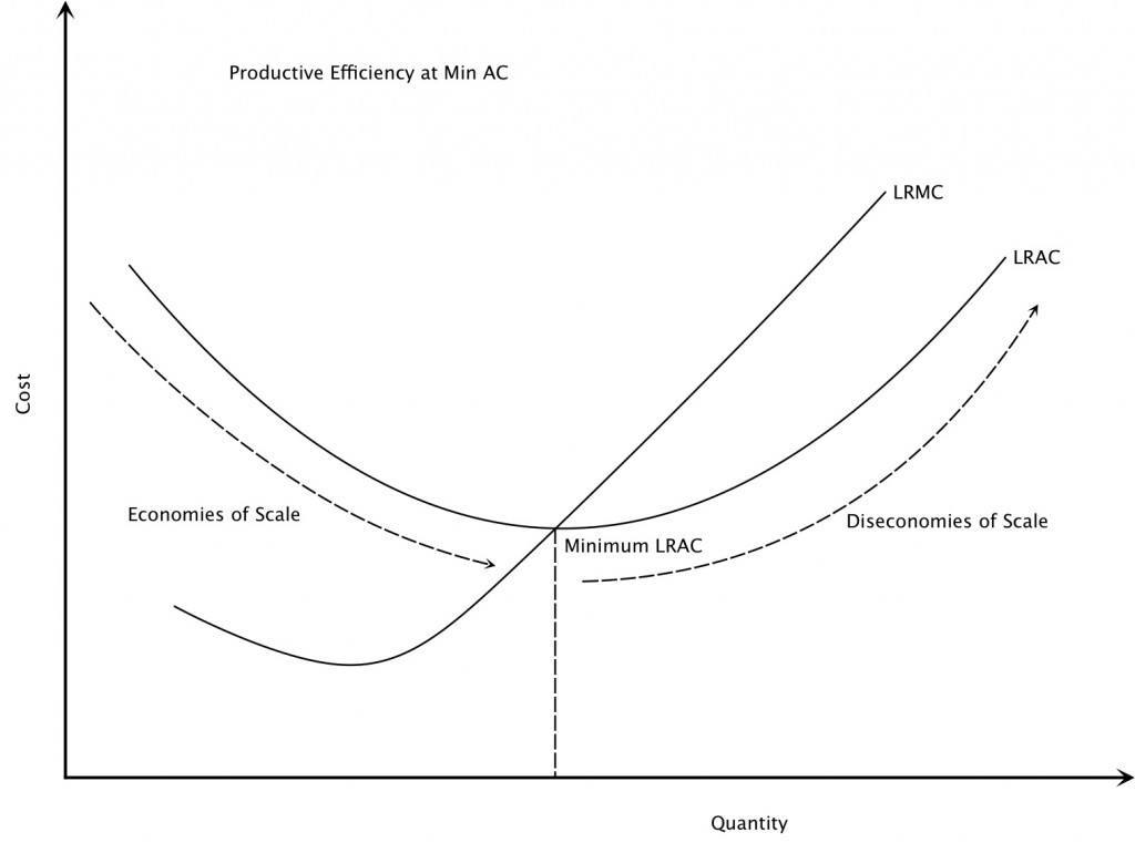
external economies of scale
- cost savings ...
- ... accruing to all firms ...
- ... as the scale of the industry increases
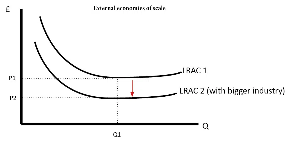
total revenue (TR)
- a firm's total sales ...
- ... or earnings ...
- ... over a given period of time
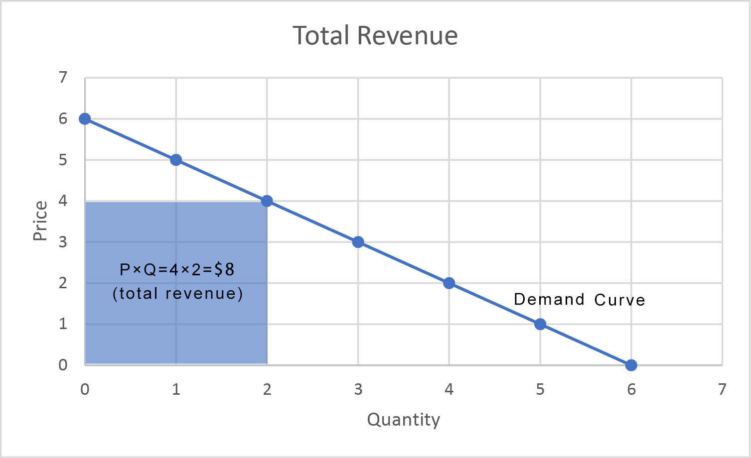
total revenue (TR)
- a firm's total sales ...
- ... or earnings ...
- ... over a given period of time

average revenue (AR)
- revenue per unit of output
$ AR = \frac{ \text{total revenue} }{ \text{output} } $
marginal revenue (MR)
- the additional ...
- ... or extra revenue ...
- ... gained from the sale of ...
- ... one more unit of output
$MR = \frac{ \Delta \text{total revenue} }{ \Delta \text{output} }$
or
$MR = \frac{ \Delta TR }{ \Delta Q }$
price taker
- a firm that is not able ...
- ... to influence market price
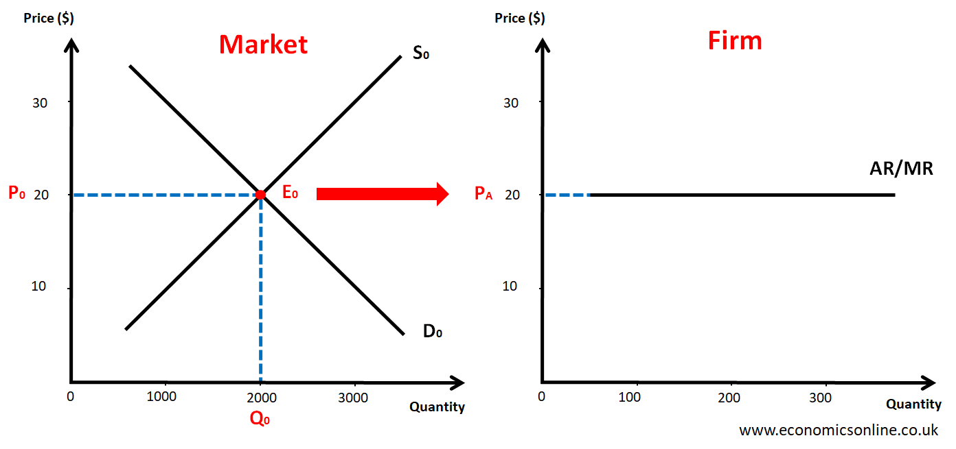
price maker
- a firm that can choose ...
- ... what price to sell its goods ...
- ... in the market
profit
- the difference between ...
- ... total revenue and ...
- ... total costs
normal profit
- a cost of production that ...
- ... is just sufficient for a firm to ...
- ... keep operating in a particular industry
supernormal profit
- that which is earned ...
- ... above normal profit
subnormal profit
- that which is earned ...
- ... below normal profit
Chapter 35: Different market structures
- market structure
- perfect competition
- imperfect competition
- monopolistic competition
- oligopoly
- barriers to entry
- pure monopoly
- natural monopoly
Chapter 35: Different market structures
- concentration ratio
- predatory pricing
- limit pricing
- collusion
- barrier to exit
- shut-down price
- price competition
- non-price competition
Chapter 35: Different market structures
- kinked demand curve
- price rigidity
- price leadership
- cartel
- X-efficiency
- contestable market
- contestability
- deregulation
market structure
- the way in which a market is organised ...
- ... in terms of certain characteristics ...
- ... which can be used to explain ...
- ... the behaviour of firms ...
- ... in a market
market structure
| Market Structure | Number of buyers and sellers | Degree of product differentiation | Degree of control over price |
|---|---|---|---|
| Monopolistic Competition | Many buyers and sellers | Some | Some |
| Oligopoly | Few sellers and many buyers | Some | Some |
| Duopoly | Two sellers and many buyers | Complete | Complete |
| Monopoly | One seller and many buyers | Complete | Complete |
perfect competition
- an ideal market structure that has :
- many buyers and sellers
- identical products
- no barriers to entry
- sometimes referred to as total competition
perfect competition
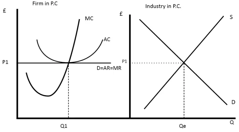
imperfect competition
- any market structure ...
- ... except for perfect competition
monopolistic competition
- a market structure where there :
- are many firms
- differentiated products
- few barriers to entry
monopolistic competition (short-run)

monopolistic competition (short-run)
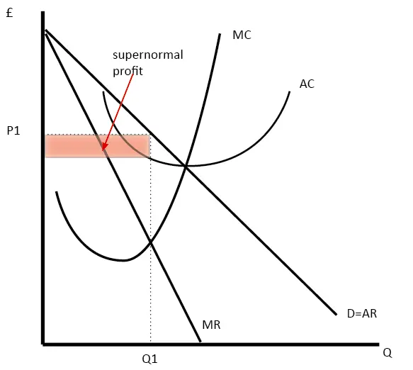
monopolistic competition (long-run)
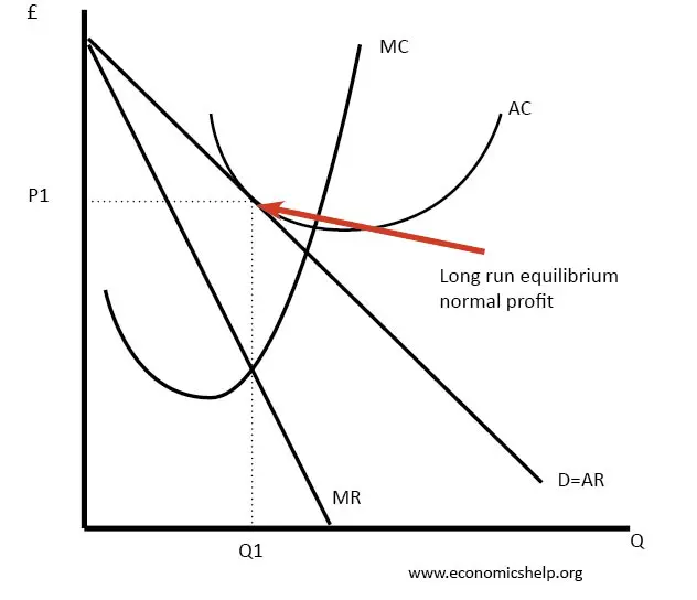
oligopoly
- a market structure with
- few firms
- high barriers to entry
oligopoly

barriers to entry
- restrictions that ...
- ... prevent new firms ...
- ... entering an industry
pure monopoly
- where there is just ...
- ... one seller in the market
pure monopoly
natural monopoly
- where with falling long-run average costs, ...
- ... it makes sense to have only one firm ...
- ... providing the good or service
concentration ratio
- a measure of the combined market share ...
- ... of the biggest three, four or five firms ...
- ... in a market
predatory pricing
- where a firm sells its goods ...
- ... below average variable cost ...
- ... to force competitors out of the market
limit pricing
- where firms deliberately lower prices and ...
- ... abandon a policy of profit maximisation ...
- ... to stop new firms entering a market
collusion
- an anti-competitive action ...
- ... by producers
barrier to exit
- a restriction that prevents ...
- ... a firm leaving a market
shut-down price
- a firm will stop production ...
- ... when price falls ...
- ... below average variable cost
price competition
- where firms compete on price ...
- ... to attract customers
non-price competition
- when firms use methods other than price ...
- ... to attract customers ...
- ... from rival producers
kinked demand curve
- a traditional model ...
- ... of a firm's behaviour ...
- ... in oligopoly
price rigidity
- where prices are unchanged ...
- ... despite a change in costs
price leadership
- a situation in a market whereby ...
- ... a particular firm has ...
- ... the power to change prices, ...
- ... the result of which is that ...
- ... competitors follow this lead
cartel
- a formal agreement between firms ...
- ... to limit competition ...
- ... by limiting output ...
- ... or fixing prices
X-efficiency
- where the firm's costs are ...
- ... above those experienced in ...
- ... a more competitive market
contestable market
- a market where ...
- ... entry is free and ...
- ... exit is costless
contestability
- the extent to which ...
- ... barriers to entry into a market are free ...
- ... and exit from the market is costless
deregulation
- when barriers to entry ...
- ... into an industry ...
- ... are removed
Chapter 36: Growth and survival of firms
- conglomerate
- economies of scope
- diversification
- horizontal integration
- vertical integration
- principal-agent problem
conglomerate
- a company with ...
- ... a large number of ...
- ... diversified businesses
BASF (Germany) : Chemicals, plastics, performance chemicals, catalysts,
coatings, crop technology, crude oil and natural gas exploration and production
TotalEnergies (France) : Petroleum, natural gas, LNG, oil refining, chemicals, solar,
biomass
economies of scope
- where a reduction in ...
- ... average total cost ...
- ... is made possible by ...
- ... a firm changing the ...
- ... different goods it produces
diversification
- where a firm grows through ...
- ... the production or sale of ...
- ... a wide range of ...
- ... different products
horizontal integration
- where a firm ...
- ... merges or acquires another ...
- ... in the same line of business
vertical integration
- where a firm ...
- ... grows by producing ...
- ... backwards or forwards ...
- ... in its supply chain
principal-agent problem
- where one person (the agent) ...
- ... makes decisions ...
- ... on behalf of ...
- ... another person (the principal)
Chapter 37: Differing objectives and policies of firms
- profit satisficing
- sales maximisation
- cross-subsidisation
- revenue maximisation
objectives of firms
- sales maximisation
- revenue maximisation
- satisficing
- profit maximisation
- survival / loss minimisation
profit maximisation

profit maximisation

profit maximisation

profit maximisation

profit maximisation

profit maximisation
slope of TC and TR
| Q1 | Q2 | Q3 | |
| slope of TC | 0.8 | 0.5 | 0.8 |
| slope of TR | 1.2 | 1.1 | 0.8 |
profit maximisation

profit satisficing
- a firm's objective to ...
- ... make a reasonable or ...
- ... minimum level of profit
sales maximisation
- a firm's objective to ...
- ... maximise the ...
- ... volume of sales
cross-subsidisation
- profits ...
- ... from one part of a firm are ...
- ... used to offset losses ...
- ... made elsewhere in the business
revenue maximisation
- a firm's objective to ...
- ... maximise total revenue
price discrimination
monopoly

price discrimination
monopoly

price discrimination

Part 8: Government microeconomic intervention
- Government policies to achieve efficient resource allocation and correct market failure
- Equity and redistribution of income and wealth
- Labour market forces and government intervention
Chapter 38: Government policies to achieve efficient resource allocation and correct market failure
- regulations
- property rights
- pollution permits
- provision of information
- production quotas
- 'nudge' theory
- nationalisation
- government failure
regulations
- a wide range of legal and other restrictions that come from government or regulatory bodies
property rights
- where owners have a right to decide how their assets may be used.
pollution permits
- a form of licence given by governments that allows a firm to pollute up to a given level.
provision of information
- when governments directly provide information to correct market failure.
production quotas
- a physical limit on what can be produced
'nudge' theory
- influencing choice by 'nudging' individuals towards making more effective decisions.
nationalisation
- when a government takes over a private sector business and transfers it to state ownership
government failure
- where government intervention to correct market failure leads to a net loss of economic welfare
Chapter 39: Equity and redistribution of income and wealth
- equality
- extreme poverty
- relative poverty
- means-tested benefits
- poverty trap
- universal benefits
- universal basic income
- negative income tax
equality
- where everyone is treated in the same way.
extreme poverty
- where a household exists on less than $1.90 a day.
relative poverty
- where household income is 50% or less than the average income.
means-tested benefits
- benefits that are paid only to those whose incomes fall below a certain level.
poverty trap
- where an individual or a family are better off on means-tested benefits rather than working.
universal benefits
- benefits available to all irrespective of income or wealth.
universal basic income
- a regular unconditional cash payment made by the government.
negative income tax
- money paid out by the government to those earning below an agreed annual fixed benefit limit.
Chapter 40: Labour market forces and government intervention
- marginal revenue product (MRP)
- trade unions
- monopsony
- wage differentials
- transfer earnings
- economic rent
marginal revenue product (MRP)
- the addition to total revenue as a result of employing one more worker.
trade unions
- an organisation of workers that aims to protect and enhance the well-being of its members through collective negotiations with employers and government.
monopsony
- where there is a single buyer in a market
wage differentials
- difference in pay between workers with different skills and responsibilities.
transfer earnings
- the amount that is earned by a factor of production in its best alternative use.
economic rent
- a payment made to a factor of production above that which is necessary to keep it in its current use.
Part 9: The macroeconomy
- The circular flow of income
- Economic growth and sustainability
- Employment and unemployment
- Money and banking
Chapter 41: The circular flow of income
- multiplier
- marginal propensity to save
- marginal propensity to consume
- aggregate expenditure
- marginal propensity to import
- consumption
- average propensity to consume (apc)
- average propensity to import
- aggregate expenditure
Chapter 41: The circular flow of income
- consumption function
- savings function
- autonomous investment
- induced investment
- accelerator theory
- capital-output ratio
- inflationary gap
- deflationary gap
multiplier
- a numerical estimate ...
- ... of a change in spending ...
- ... in relation to the ...
- ... final change in spending
$ \text{multiplier} = \frac{ \text{change in income} }{ \text{change in injection} } $
$= \frac{ {\Delta Y} }{ \Delta J }$
multiplier
$ \text{multiplier} = \frac{ 1 }{ \text{marginal propensity to withdraw} } $
marginal propensity to save
- the proportion of ...
- ... extra income which ...
- ... is saved
marginal propensity to consume
- the proportion of ...
- ... extra income that ...
- ... is spent
aggregate expenditure
- the total amount spent ...
- ... in the economy ...
- ... at different levels of income
marginal propensity to import
- the proportion of ...
- ... extra income spent ...
- ... on imports
consumption
- spending by ...
- ... households on ...
- ... goods and services
average propensity to consume (apc)
- the proportion of ...
- ... income that is ...
- ... consumed
average propensity to import
- the proportion of ...
- ... income that is ...
- ... spent on imports
- the proportion of ...
- ... income that is ...
- ... spent on imports
Keynesian 45° diagram
Keynesian 45° diagram
at equilibrium

consumption function
- the relationship between ...
- ... income and consumption
$C = a + bY$
where $C$ is consumption,
$Y$ is disposable income,
$a$ is autonomous consumption,
$b$ is the marginal propensity to consume ($mpc$)
savings function
- the relationship between ...
- ... income and saving
$S = -a + sY$
where $S$ is saving,
$s$ is the marginal propensity to save,
$a$ is autonomous dissaving
macroeconomic models
simple 2-sector model (closed economy)
- agents : households and firms
- withdrawal : savings ($S$)
injection : investment ($I$) - $ \text{multiplier} = \frac{1}{mps} $ or $ \text{multiplier} = \frac{1}{1 - mpc} $
- where $ mpc = \frac{ \text{change in consumption} }{ \text{change in income} } = \frac{ \Delta C }{ \Delta Y }$
- equilibrium income will occur :
$Y = C + I$ : output = aggregate expenditure
$I = S$ : injection = withdrawal
macroeconomic models
simple 3-sector model (closed economy)
- agents : households, firms and government
- withdrawal : savings ($S$), taxes ($T$)
injection : investment ($I$), gov. spending ($G$) - $ \text{multiplier} = \frac{1}{mps + mrt} $
- where $mrt$ : marginal rate of taxation
- equilibrium income will occur :
$Y = C + I + G$ : output = aggr. expenditure
$I + G= S + T$ : injection = withdrawal
macroeconomic models
simple 4-sector model (open economy)
- agents : households, firms, government, foreign trade sector
- withdrawal : $S$, $T$, import ($M$)
injection : $I$, $G$, exports ($X$) - $ \text{multiplier} = \frac{1}{mps + mrt + mpm} $
where $mpm$ : marginal propensity to import - equilibrium income will occur :
$Y = C + I + G + (X-M)$
$I + G + X= S + T + M$
autonomous investment
- investment that is made ...
- ... independent of income
induced investment
- investment that is made ...
- ... in response to changes in income
accelerator theory
- a model that suggests ...
- ... investment depends on the ...
- ... rate of change in income
capital-output ratio
- a measure of the ...
- ... amount of capital used to ...
- ... produce a given amount, or value, ...
- ... of output
inflationary gap
- the excess of ...
- ... aggregate expenditure ...
- ... over potential output ...
- ... (equivalent to a positive output gap)
Keynesian 45° diagram
inflationary gap

deflationary gap
- a shortage of ...
- ... aggregate expenditure so that ...
- ... potential output is not reached ...
- ... (equivalent to a negative output gap)
Keynesian 45° diagram
deflationary gap

Keynesian 45° diagram
eliminating the deflationary gap through government intervention

application: marginal propensity to consume
- In 2022 it was estimated that an increase in government spending of 25 billion dollar in an economy would eventually result in an increase in the country's national income of 100 billion dollar.
- Based on this information, calculate the marginal propensity to consume (MPC) in this economy.
- Show your workings.
solution: marginal propensity to consume
- marginal propensity to consume is the proportion of individual's, firm's income spent on consumption
- multiplier $= \frac{ 100 \text{ billion dollar} }{ 25 \text{ billion dollar} } = 4$
- $\frac{1}{1 - mpc} = 4 \iff 1 - mpc = 0.25 $
- $ mpc = 0.75$
Chapter 42: Economic growth and sustainability
- actual economic growth
- potential economic growth
- output gap
- negative output gap
- positive output gap
- business cycle
- depression
Chapter 42: Economic growth and sustainability
- gig economy
- sustainable economic growth
- climate change
- greenhouse gases
- global warming
- polluter pays principle
actual economic growth
- an increase ...
- ... in real GDP

potential economic growth
- an increase ...
- ... in the productive capacity ...
- ... of the economy

output gap
- a gap between ...
- ... actual and ...
- ... potential output

the business cycle.
negative output gap
- a situation where ...
- ... actual output is ...
- ... below potential output
$ \text{ actual output } < \text{ potential output } $
positive output gap
- a situation where ...
- ... actual output is ...
- ... above potential output
$ \text{ actual output } > \text{ potential output } $
business cycle (or trade cycle)
- fluctuations in ...
- ... economic activity
business cycle (or trade cycle)

depression
- a fall ...
- ... in real GDP that ...
- ... lasts several years

gig economy
- a labour market based on ...
- ... short-term contracts

Deliveroo food
sustainable economic growth
- economic growth that ...
- ... does not threaten ...
- ... future generations' ability to ...
- ... experience economic growth
climate change
- a change ...
- ... in the weather ...
- ... of a region over ...
- ... a period of time
greenhouse gases
- carbon dioxide, ...
- ... methane, ...
- ... nitrous oxide
global warming
- a rise ...
- ... in the temperature ...
- ... of the world's atmosphere ...
- ... arising from the emission of ...
- ... greenhouse gases
polluter pays principle
- a policy ...
- ... that makes those responsible ...
- ... for causing damage to the environment ...
- ... pay for that damage
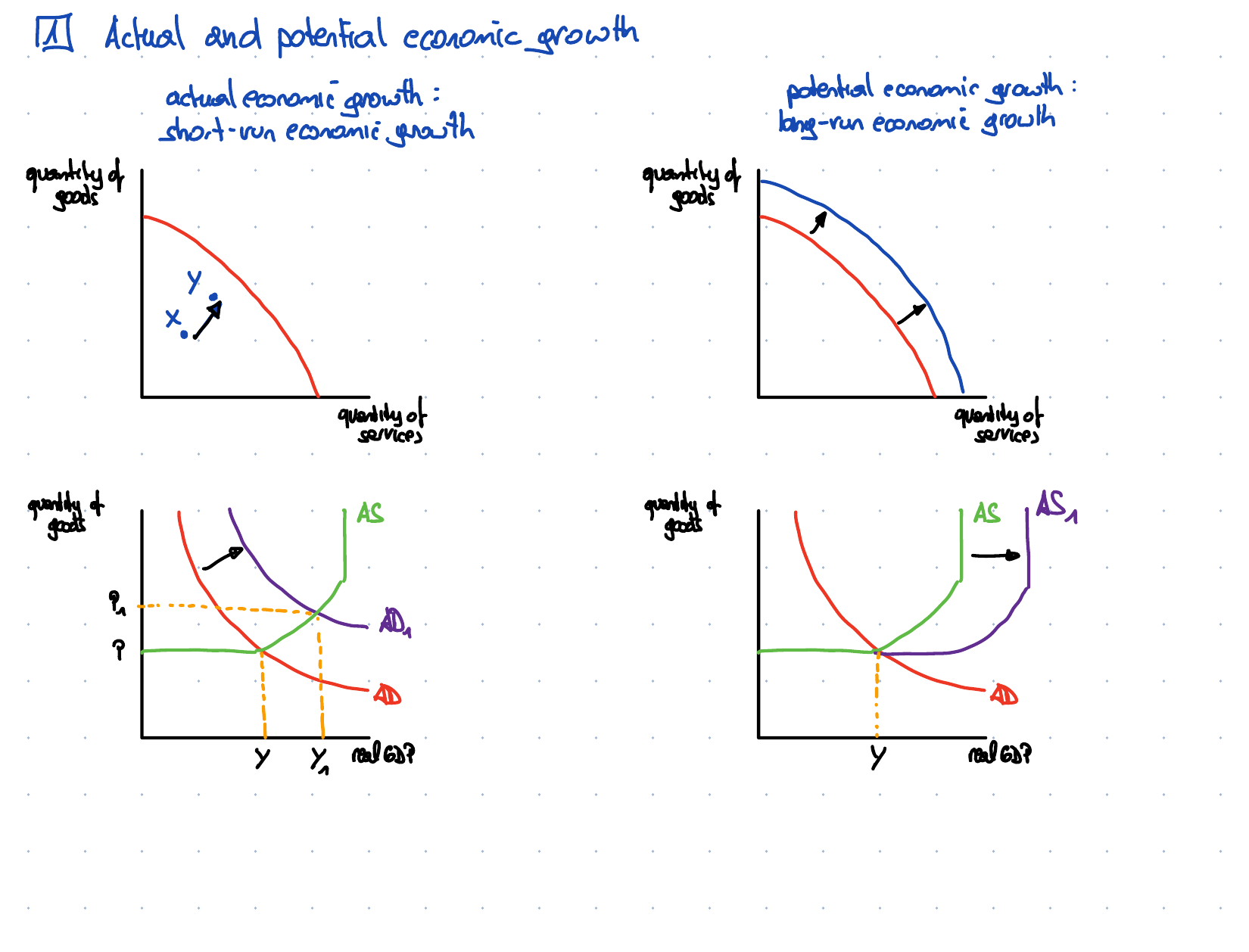
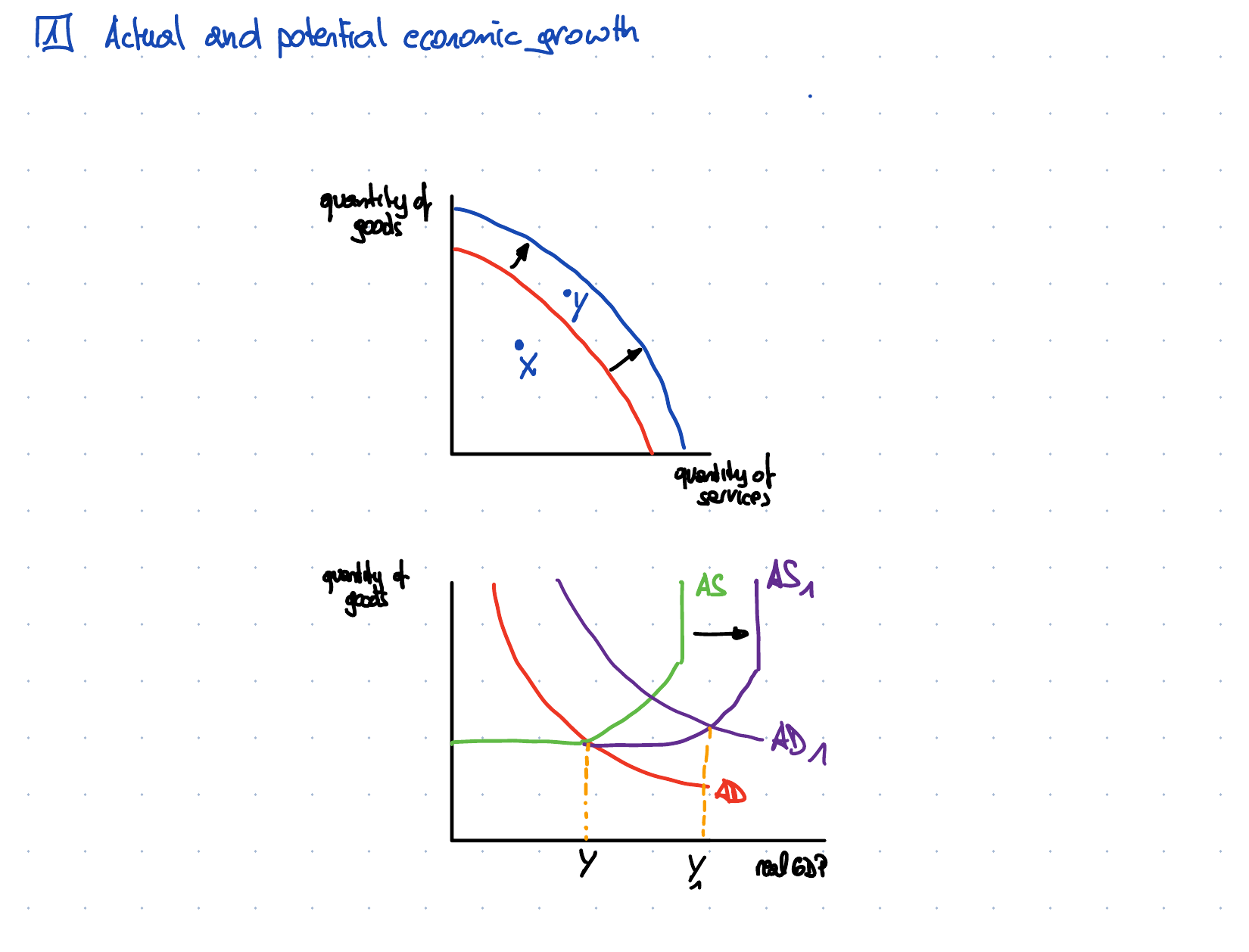
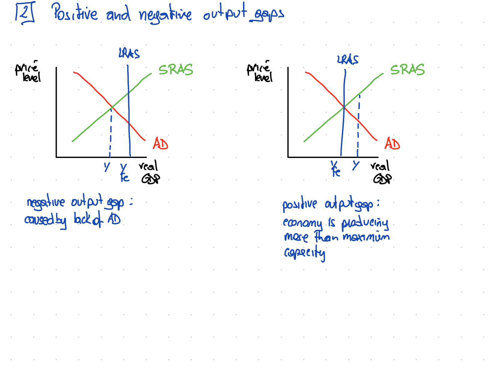
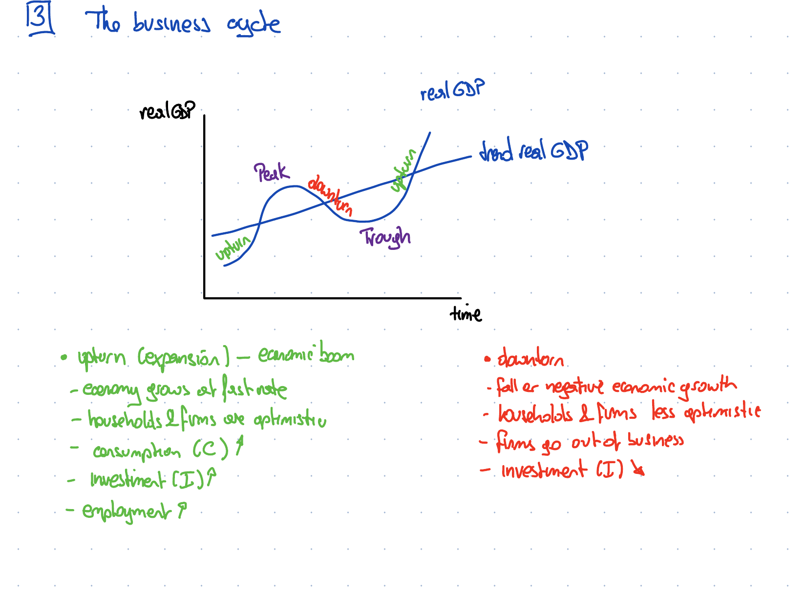
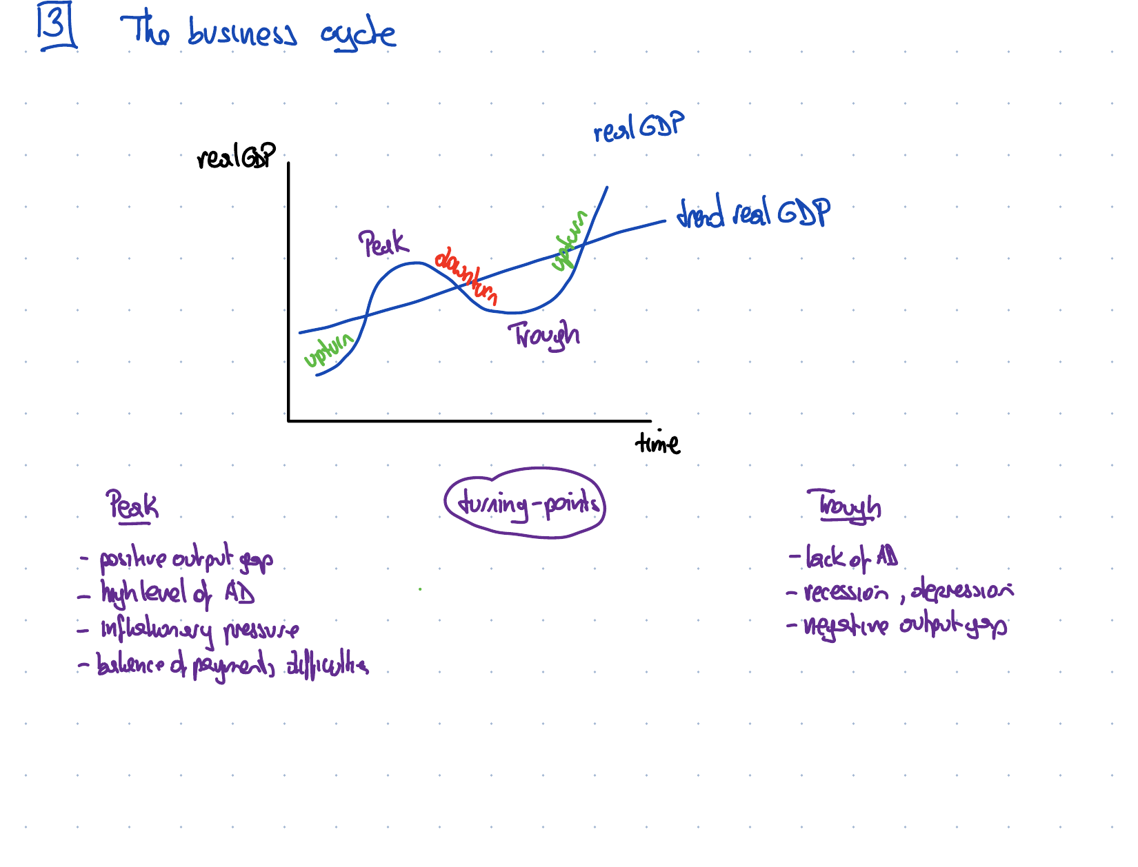

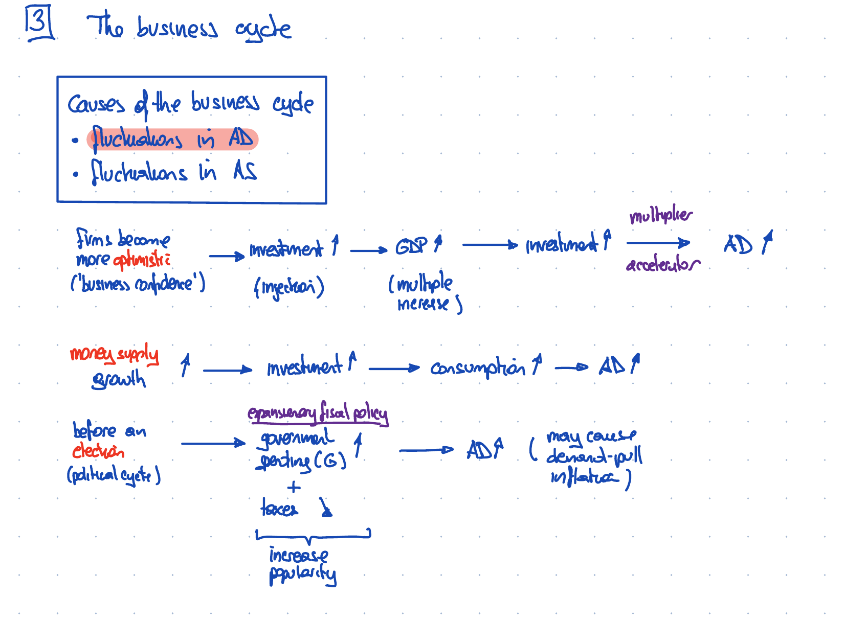
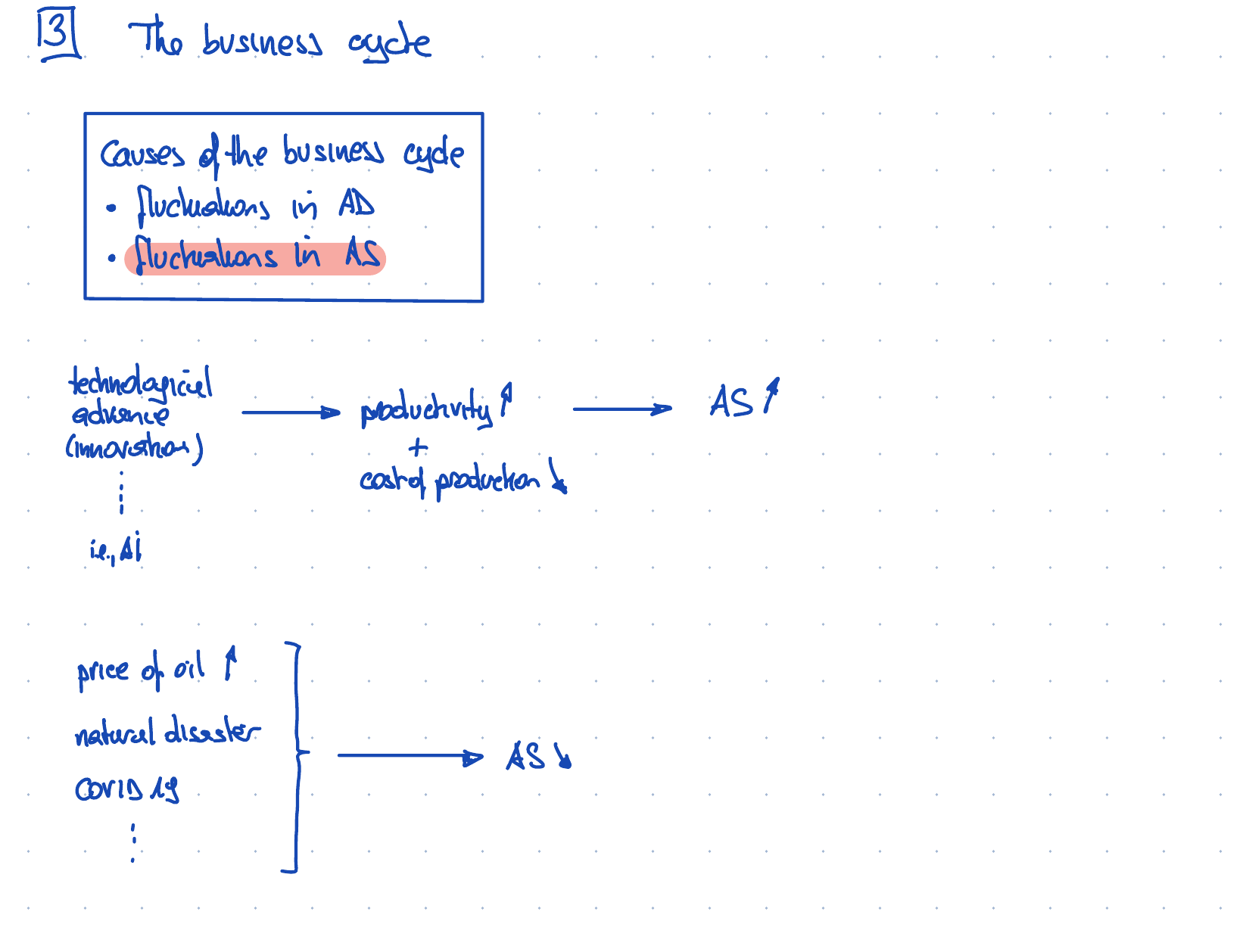
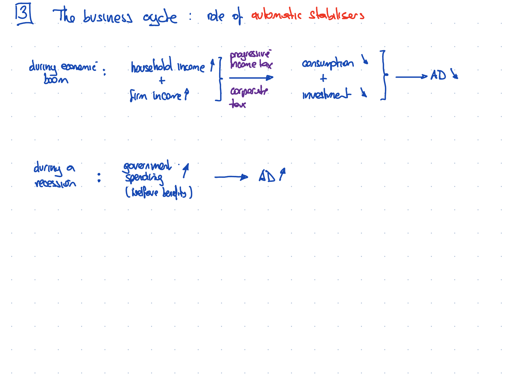

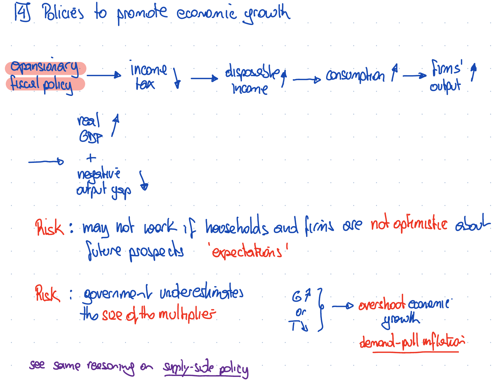
Chapter 43: Employment and unemployment
- full employment
- equilibrium unemployment
- voluntary unemployment
- disequilibrium unemployment
- natural rate of unemployment
- hysteresis
- long-term unemployed
- labour mobility
- self-employed
- occupational mobility
- geographical mobility
equilibrium unemployment

disequilibrium unemployment

equilibrium and disequilibrium unemployment

full employment
- the level of employment ...
- ... corresponding to where ...
- ... all who wish to work ...
- ... have found jobs, excluding ...
- ... frictional unemployment
equilibrium unemployment
- the unemployment which exists ...
- ... when the labour market is in equilibrium.
- It includes :
- voluntary
- frictional
- structural unemployment
voluntary unemployment
- unemployment that arises ...
- ... when workers are not willing to work ...
- ... at the current wage rate
disequilibrium unemployment
- unemployment that arises ...
- ... when the aggregate supply of labour ...
- ... is greater than the ...
- ... aggregate demand for labour ...
- ... at the current wage rate
$ ASL > ADL $
natural rate of unemployment
- the rate of unemployment that exists ...
- ... when the aggregate demand for labour ...
- ... equals ...
- ... the aggregate supply of labour ...
- ... at current wage rate and price level
$ ADL = ASL $
natural rate of unemployment
determining supply-side factors
- value of unemployment benefits
- minimum wage
- quality of education
- impact on unemployed workers
- information about
- job vacancies
- workers' skills
- qualifications
hysteresis
- unemployment causing unemployment ...
- ... due to workers becoming ...
- ... deskilled and demotivated ...
- ... when they are out of work ...
- ... for a long time
long-term unemployed
- those who have been unemployed ...
- ... for a year or longer
labour mobility
- ability of workers to change ...
- ... where they work and ...
- ... in which occupation
self-employed
- those working for themselves
occupational mobility
- the ability of workers ...
- ... to move from one occupation ...
- ... to another occupation
geographical mobility
- the ability of workers ...
- ... to move to a job ...
- ... in a different location
Chapter 44: Money and banking
- money
- double coincidence of wants
- money supply
- narrow money
- broad money
- quantity theory of money
- Fisher equation
Chapter 44: Money and banking
- demand deposit account
- savings deposit account
- government securities
- equities
- overdraft
- loan
- reserve ratio
Chapter 44: Money and banking
- capital ratio
- liquidity
- bank credit multiplier
- quantitative easing
- total currency flow
- economic and monetary union
- liquidity preference
Chapter 44: Money and banking
- transactions motive
- precautionary motive
- active balances
- speculative motive
- idle balances
- liquidity trap
money
- an item which is generally acceptable as a means of payment
double coincidence of wants
- a situation where two people each have something the other one wants
money supply
- the total amount of money in an economy.
narrow money
- money that can be spent directly.
broad money
- money used for spending and saving.
quantity theory of money
- the theory that links inflation in an economy to changes in the money supply
Fisher equation
- the statement that MV = PT.
demand deposit account
- a bank account that allows the holder to make and receive payments.
savings deposit account
- a bank account which pays interest and may require notice to be given before money can be withdrawn from it
government securities
- bills and bonds issued by the government to raise money.
equities
- shares in firms
overdraft
- permission to spend more than is in a demand deposit account
loan
- a sum of money lent at an agreed rate of interest for a specific time period.
reserve ratio
- the proportion of liquid assets to total liabilities.
capital ratio
- a bank's available financial capital as a percentage of its riskier assets.
liquidity
- the ability to turn an asset into cash quickly and without loss.
bank credit multiplier
- the process by which banks can make more loans than deposits available
quantitative easing
- a situation where a central bank buys government and private securities from the private sector in order to increase the money supply and so stimulate economic activity
total currency flow
- the net amount of money that flows into or out of the country as a result of international transactions.
economic and monetary union
- co-ordination of policies and the operation of a single currency by a group of countries.
liquidity preference
- a Keynesian concept that explains why people demand money
transactions motive
- the desire to hold money for the day-to-day buying of goods and services
precautionary motive
- a reason for holding money for unexpected or unforeseen events
active balances
- the amount of money held by households or firms for possible near-future use.
speculative motive
- a reason for holding money with a view to make future gains from buying financial assets.
idle balances
- the amount of money held temporarily as the returns from holding financial assets are too low.
liquidity trap
- a situation where interest rates cannot be reduced any more in order to stimulate an upturn in economy activity
Part 10 : Government macroeconomic intervention
- Government macroeconomic policy objectives
- Links between macroeconomic problems and their interrelatedness
- Effectiveness of policy options to meet all macroeconomic objectives
Chapter 45: Government macroeconomic policy objectives
- inflation
- balance of payments
- unemployment
- economic growth
- economic development
- sustainability
- redistribution of income and wealth
Chapter 46: Links between macroeconomic problems and their interrelatedness
- Phillips curve
- expectations-augmented Phillips curve
Phillips curve
- a curve that shows the relationship between the unemployment rate and the inflation rate over a period of time.
expectations-augmented Phillips curve
- a diagram that shows that while there may be a trade-off between unemployment and inflation in the short run, there is no trade-off in the long run.
Chapter 47: Effectiveness of policy options to meet all macroeconomic objectives
- crowding out
- crowding in
- Laffer curve
- government macroeconomic failure
- counter-cyclically
crowding out
- the idea that higher public sector spending will just replace private sector spending.
crowding in
- the idea that higher public sector spending will increase private sector spending.
Laffer curve
- a curve showing tax revenue rising at first as the tax rate is increasing and then falling beyond a certain rate.
government macroeconomic failure
- government intervention reducing rather than increasing economic performance.
counter-cyclically
- going against the fluctuations in economic activity
Part 11 : International economic issues
- Policies to correct disequilibrium in the balance of payments
- Exchange rates
- Economic development
- Characteristics of countries at different levels of development
- Relationship between countries at different levels of development
- Globalisation
Chapter 48: Policies to correct disequilibrium in the balance of payments
- net errors and omissions
- expenditure switching policy
- expenditure reducing policy
net errors and omissions
- a figure included to ensure the balance of payments balances; sometimes called the balancing item.
expenditure switching policy
- policy tools designed to encourage people to switch from buying foreign-produced products to buying domestically produced products.
expenditure reducing policy
- policy tools designed to reduce imports and increase exports by reducing demand
Chapter 49: Exchange rates
- real exchange rate
- trade-weighted exchange rates
- fixed exchange rate
- devaluation
- revaluation
- managed system
- Marshall-Lerner condition
- J curve effect
real exchange rate
- a currency's value in terms of its real purchasing power.
trade-weighted exchange rates
- the price of one currency against a basket of currencies
fixed exchange rate
- an exchange rate set by the government and maintained by the central bank.
devaluation
- a decision by the government to lower the international price of the country's currency
revaluation
- a decision by the government to raise the international price of the country's currency.
managed system
- where the exchange rate is influenced by state intervention.
Marshall-Lerner condition
- the requirement that for a fall in the exchange rate to be successful in reducing a current account deficit, the sum of the price elasticities of demand for exports and imports must be greater than 1
J curve effect
- a fall in the exchange rate causing an increase in a current account deficit before it reduces it due to the time it takes for demand to respond.
Chapter 50: Economic development
- poverty cycles
- development traps
- purchasing power parity (PPP)
- Human Development Index (HDI)
- Measurable Economic Welfare (MEW)
- Multidimensional Poverty Index (MPI)
- Kuznets curve
- shadow economy
poverty cycles
- the links between, for example, low income, low savings, low investment and low productivity.
development traps
- restrictions on the growth of developing economies that arise from low levels of savings and investment
purchasing power parity (PPP)
- a way of comparing international living standards by using an exchange rate based on the amount of each currency needed to purchase the same basket of goods and services.
Human Development Index (HDI)
- a composite measure of living standards that includes GNI per head, education and life expectancy
Measurable Economic Welfare (MEW)
- a composite measure of living standards that adjusts GDP for factors that reduce living standards and factors that improve living standards
Multidimensional Poverty Index (MPI)
- a composite measure of deprivation in terms of the proportion of households that lack the requirements for a reasonable standard of living
Kuznets curve
- a curve that shows the relationship between economic growth and income inequality.
shadow economy
- the output of goods and services hidden from the authorities
Chapter 51: Characteristics of countries at different levels of development
- demographers
- birth rate
- death rate
- infant mortality rate
- net migration
- natural increase in population
- positive net migration
Chapter 51: Characteristics of countries at different levels of development
- net migration rate
- dependency ratios
- optimum population
- Lorenz curve
- primary sector
- secondary sector
- tertiary sector
demographers
- people who study changes in the structure of human populations.
birth rate
- the number of live births per thousand of the population in one year.
death rate
- the number of deaths per thousand of the population in one year.
infant mortality rate
- the number of deaths of children aged under one per thousand live births in one year.
net migration
- the difference between immigration and emigration
natural increase in population
- the number of live births exceeding the number of deaths
positive net migration
- more people coming to live in the country than people leaving the country to live
net migration rate
- the number of migrants per thousand of the population in one year.
dependency ratios
- the proportion of the economically inactive compared to the labour force
optimum population
- the size of population that maximises GDP per head
Lorenz curve
- a diagram illustrating the extent of income or wealth inequality.
primary sector
- industries involved in farming and extracting natural resources.
secondary sector
- industries that manufacture products.
tertiary sector
- industries that produce services.
Chapter 52: Relationship between countries at different levels of development
- International Monetary Fund (IMF)
- aid
- tied aid
- untied aid
- bilateral aid
- multilateral aid
- virtuous cycle
- emerging economies
- foreign direct investment (FDI)
International Monetary Fund (IMF)
- an international organisation that promotes free trade and helps countries in balance of payments difficulties.
aid
- assistance given to other countries on favourable terms.
tied aid
- aid with conditions attached.
untied aid
- aid without conditions attached.
bilateral aid
- aid given by one country to another country
multilateral aid
- aid given by international organisations to a country or countries.
virtuous cycle
- the links between, for example, an increase in investment, increase in productivity, increase in income and increase in saving.
emerging economies
- economies that are making quick progress towards becoming high-income economies
foreign direct investment (FDI)
- the setting up of production units or the purchase of existing production units in other countries.
Chapter 53: Globalisation
- globalisation
- trade blocs
- free trade area
- customs union
- monetary union
- full economic union
- trade creation
- trade diversion
globalisation
- the process by which the world is becoming increasingly interconnected through trade and other links.
trade blocs
- a regional group of countries that have entered into trade agreements
free trade area
- a trade bloc where member governments agree to remove trade restrictions among themselves.
customs union
- a trade bloc where there is free trade between member countries and a common external tariff on imports from non-members
monetary union
- a trade bloc which involves member countries operating the same currency, having one exchange rate and the same interest rate.
full economic union
- a trade bloc where there is free trade between member countries, a common external tariff, common economic policies and the same currency.
trade creation
- where high-cost domestic production is replaced by more efficiently produced imports from within the customs union
trade diversion
- where trade with a low-cost country outside a customs union is replaced by higher-cost products supplied from within the customs union.